Chapter 2 Geometric morphometrics

2.1 Load packages + data

# download most recent software version
#devtools::install_github("geomorphR/geomorph", ref = "Stable", build_vignettes = TRUE)
#devtools::install_github("mlcollyer/RRPP")

# load analysis packages
library(here)
library(StereoMorph)
library(geomorph)

## Loading required package: rgl

## Loading required package: Matrix

## 
## Attaching package: 'Matrix'

## The following objects are masked from 'package:tidyr':
## 
##     expand, pack, unpack

library(ggplot2)
library(dplyr)
library(wesanderson)

# read shape data and define number of sLMs
shapes <- readShapes("shapes")
shapesGM <- readland.shapes(shapes, nCurvePts = c(20))

# read qualitative data
qdata <- read.csv("qdata.csv",
                  header = TRUE,
                  row.names = 1)

2.2 Generalised Procrustes Analysis

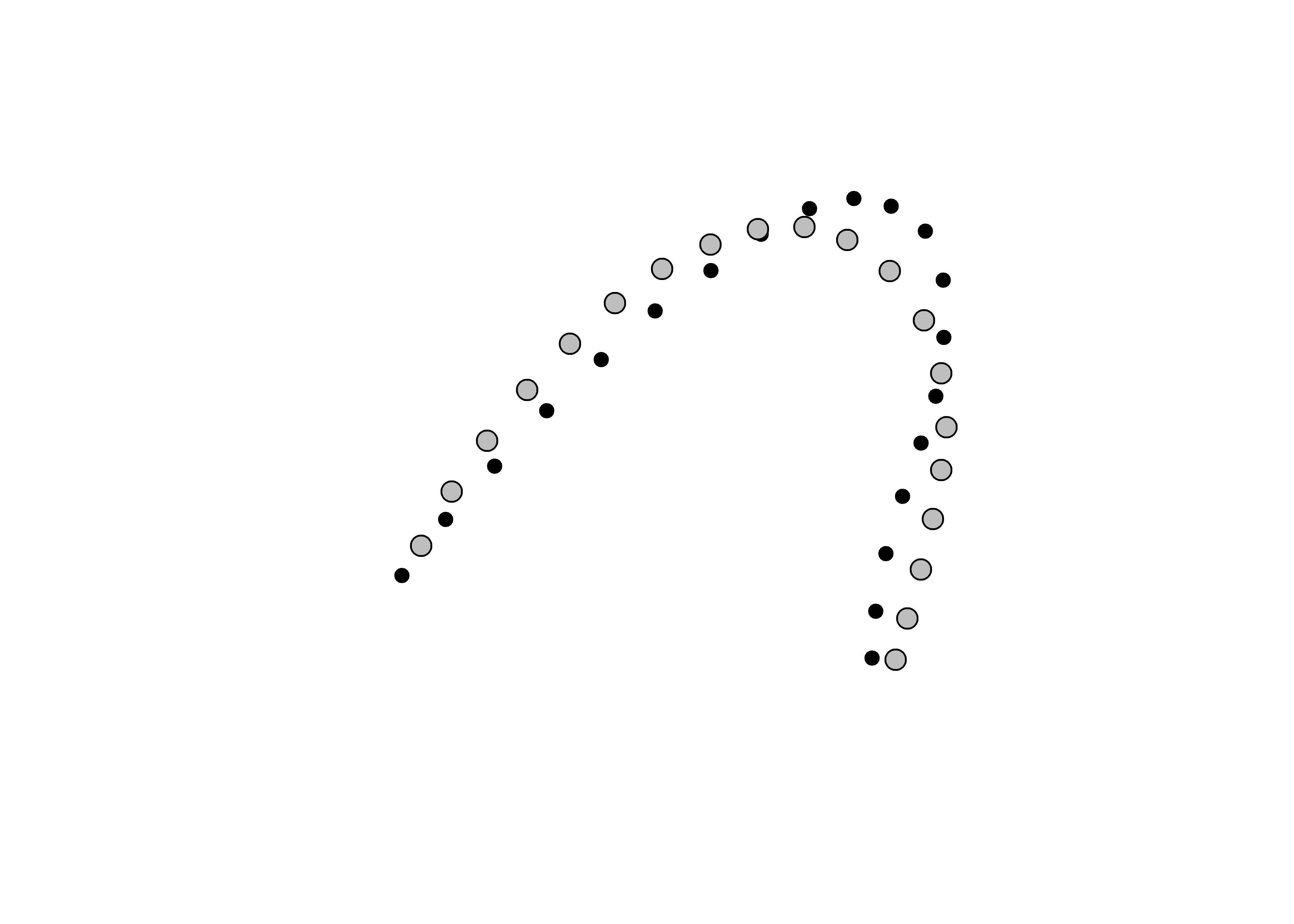
Landmark data were aligned to a global coordinate system (Kendall 1981, 1984; Slice 2001), achieved through generalized Procrustes superimposition (Rohlf and Slice 1990) performed in R 4.0.5 (R Core Development Team, 2017) using the geomorph library v. 4.0.0 (Adams et al. 2017; Adams and Otárola-Castillo 2013). Procrustes superimposition translates, scales, and rotates the coordinate data to allow for comparisons among objects (Gower 1975; Rohlf and Slice 1990). The geomorph package uses a partial Procrustes superimposition that projects the aligned specimens into tangent space subsequent to alignment in preparation for the use of multivariate methods that assume linear space (Rohlf 1999; Slice 2001).

# gpa
Y.gpa <- gpagen(shapesGM, print.progress = FALSE)
plot(Y.gpa)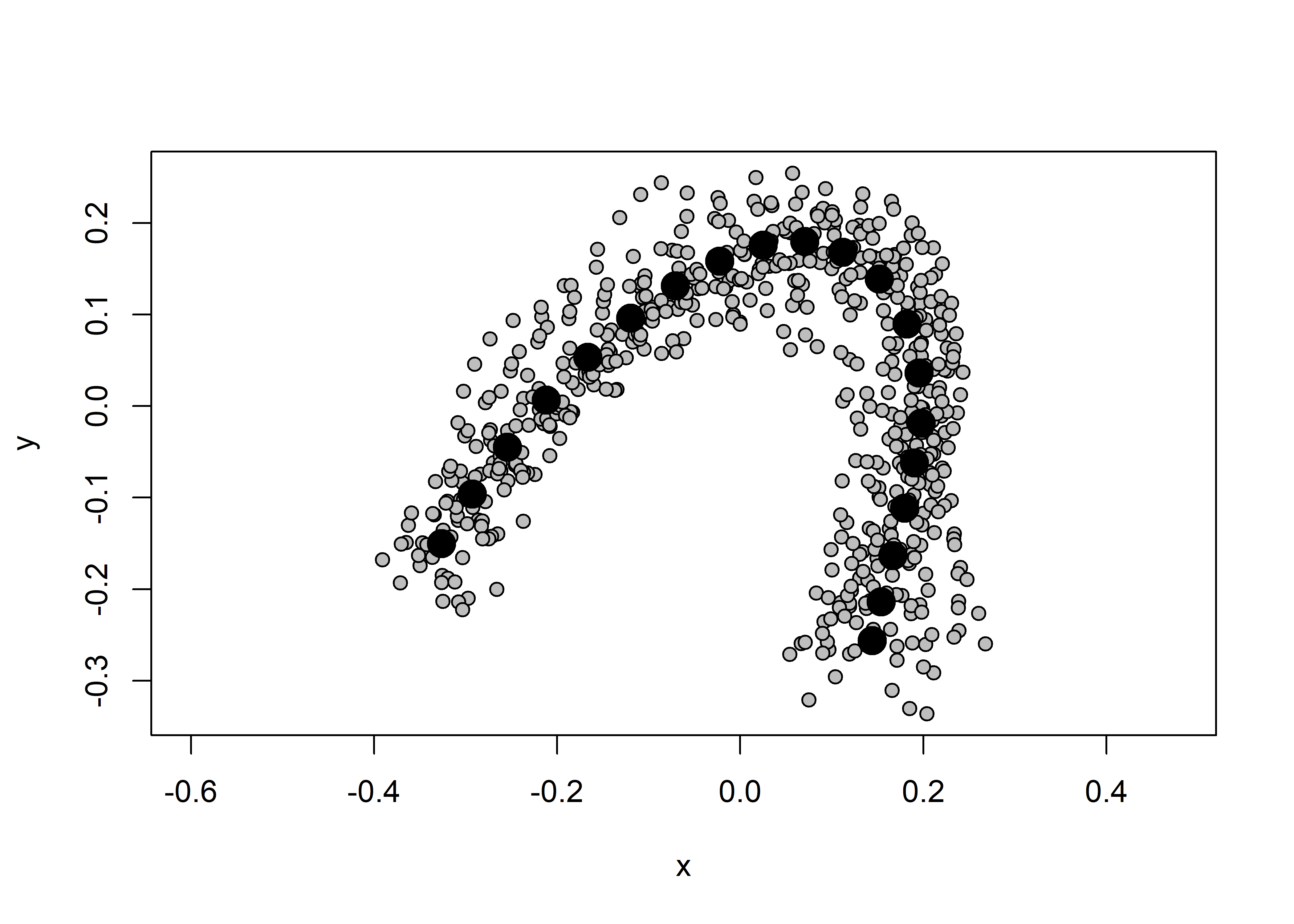

2.3 Boxplot (centroid size)

# dataframe
gdf <- geomorph.data.frame(shape = Y.gpa$coords,
                           size = Y.gpa$Csize,
                           cont = qdata$ context)

# add centroid size to qdata
qdata$csz <- Y.gpa$Csize

# attributes
csz <- qdata$csz
context <- qdata$context

# palette
pal = wes_palette("Moonrise2")

# boxplot of Perdiz arrow points by context
csz.temp <- ggplot(qdata, aes(x = context, y = csz, color = context)) +
  geom_boxplot() +
  geom_dotplot(binaxis = 'y', stackdir = 'center', dotsize = 0.3) +
  scale_color_manual(values = pal) +
  theme(legend.position = "none") +
  theme(axis.text.x = element_text(angle = 90, vjust = 0.5, hjust=1)) +
  labs(x = 'Raw Material', y = 'Centroid Size')

# render plot
csz.temp

## Bin width defaults to 1/30 of the range of the data. Pick better value with `binwidth`.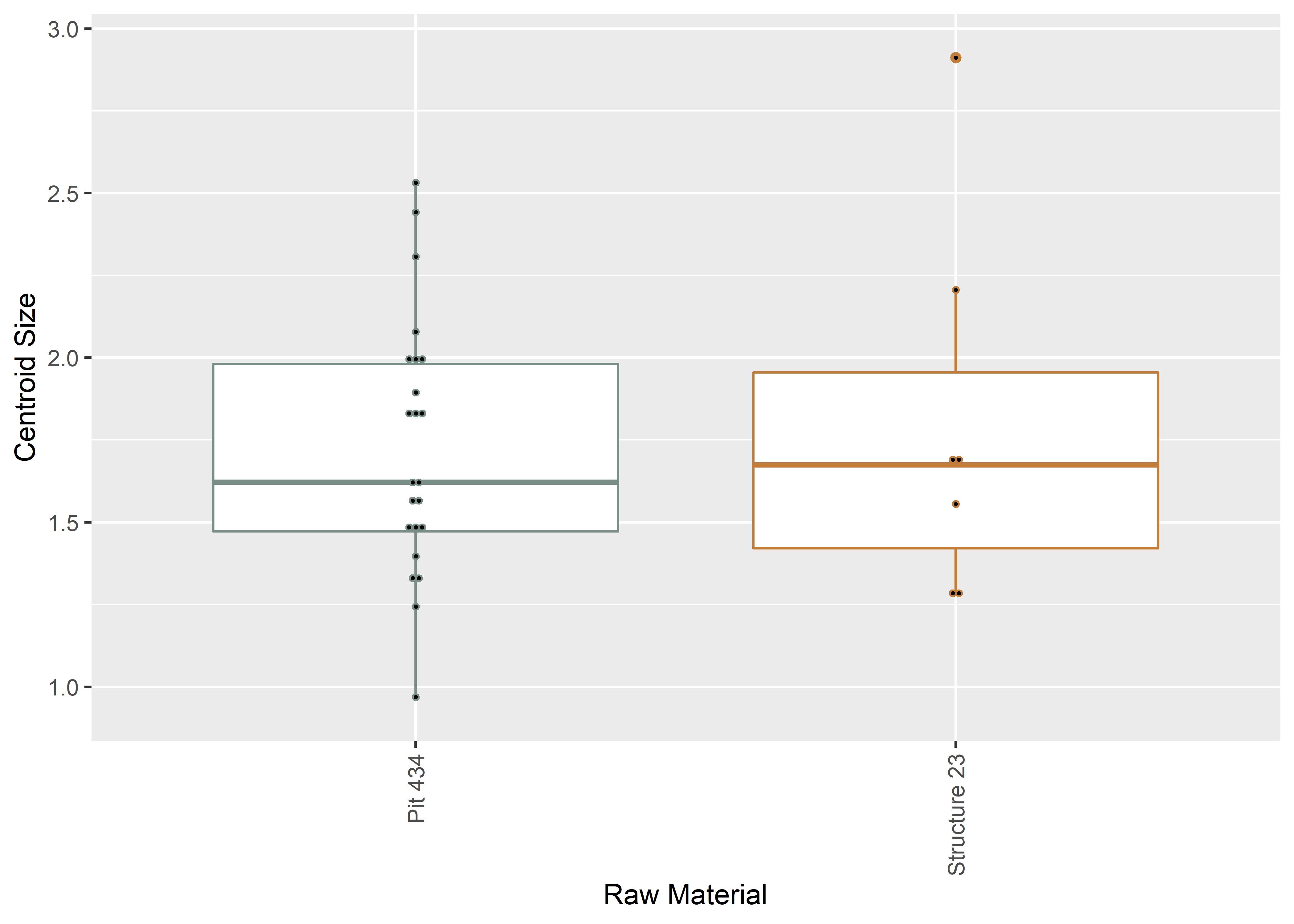

2.4 Principal Components Analysis

Principal components analysis (Jolliffe 2002) was used to visualise shape variation among the bifaces. The shape changes described by each principal axis are commonly visualized using thin-plate spline warping of a reference 3D mesh (Klingenberg 2013; Sherratt et al. 2014).

# pca
pca <- gm.prcomp(Y.gpa$coords)
summary(pca)

## 
## Ordination type: Principal Component Analysis 
## Centering by OLS mean
## Orthogonal projection of OLS residuals
## Number of observations: 30 
## Number of vectors 29 
## 
## Importance of Components:
##                            Comp1      Comp2       Comp3        Comp4        Comp5        Comp6        Comp7
## Eigenvalues            0.0371361 0.01634379 0.002105276 0.0006150787 0.0004071649 0.0002011171 0.0001378441
## Proportion of Variance 0.6491699 0.28570315 0.036801982 0.0107520889 0.0071175814 0.0035156955 0.0024096305
## Cumulative Proportion  0.6491699 0.93487306 0.971675045 0.9824271341 0.9895447155 0.9930604110 0.9954700415
##                               Comp8        Comp9       Comp10       Comp11       Comp12       Comp13       Comp14
## Eigenvalues            9.249565e-05 6.610968e-05 3.441467e-05 2.358206e-05 1.273002e-05 8.279266e-06 6.377831e-06
## Proportion of Variance 1.616901e-03 1.155652e-03 6.015971e-04 4.122341e-04 2.225314e-04 1.447285e-04 1.114898e-04
## Cumulative Proportion  9.970869e-01 9.982426e-01 9.988442e-01 9.992564e-01 9.994790e-01 9.996237e-01 9.997352e-01
##                              Comp15       Comp16       Comp17       Comp18       Comp19       Comp20       Comp21
## Eigenvalues            3.601826e-06 3.218518e-06 2.218869e-06 1.751957e-06 1.361077e-06 8.823034e-07 7.436413e-07
## Proportion of Variance 6.296292e-05 5.626238e-05 3.878768e-05 3.062567e-05 2.379275e-05 1.542340e-05 1.299947e-05
## Cumulative Proportion  9.997981e-01 9.998544e-01 9.998932e-01 9.999238e-01 9.999476e-01 9.999630e-01 9.999760e-01
##                              Comp22       Comp23       Comp24       Comp25       Comp26       Comp27       Comp28
## Eigenvalues            6.629143e-07 2.383783e-07 1.985124e-07 1.381615e-07 5.898989e-08 4.174008e-08 2.855408e-08
## Proportion of Variance 1.158830e-05 4.167051e-06 3.470163e-06 2.415178e-06 1.031193e-06 7.296515e-07 4.991491e-07
## Cumulative Proportion  9.999876e-01 9.999918e-01 9.999953e-01 9.999977e-01 9.999987e-01 9.999994e-01 9.999999e-01
##                              Comp29
## Eigenvalues            3.955376e-09
## Proportion of Variance 6.914327e-08
## Cumulative Proportion  1.000000e+00

# set plot parameters
pch.gps <- c(15,17)[as.factor(qdata$context)]
col.gps <- pal[as.factor(qdata$context)]
col.hull <- c("#798E87","#C27D38")

# pca plot
pc.plot <- plot(pca,
                asp = 1,
                pch = pch.gps,
                col = col.gps)
shapeHulls(pc.plot,
           groups = qdata$context,
           group.cols = col.hull)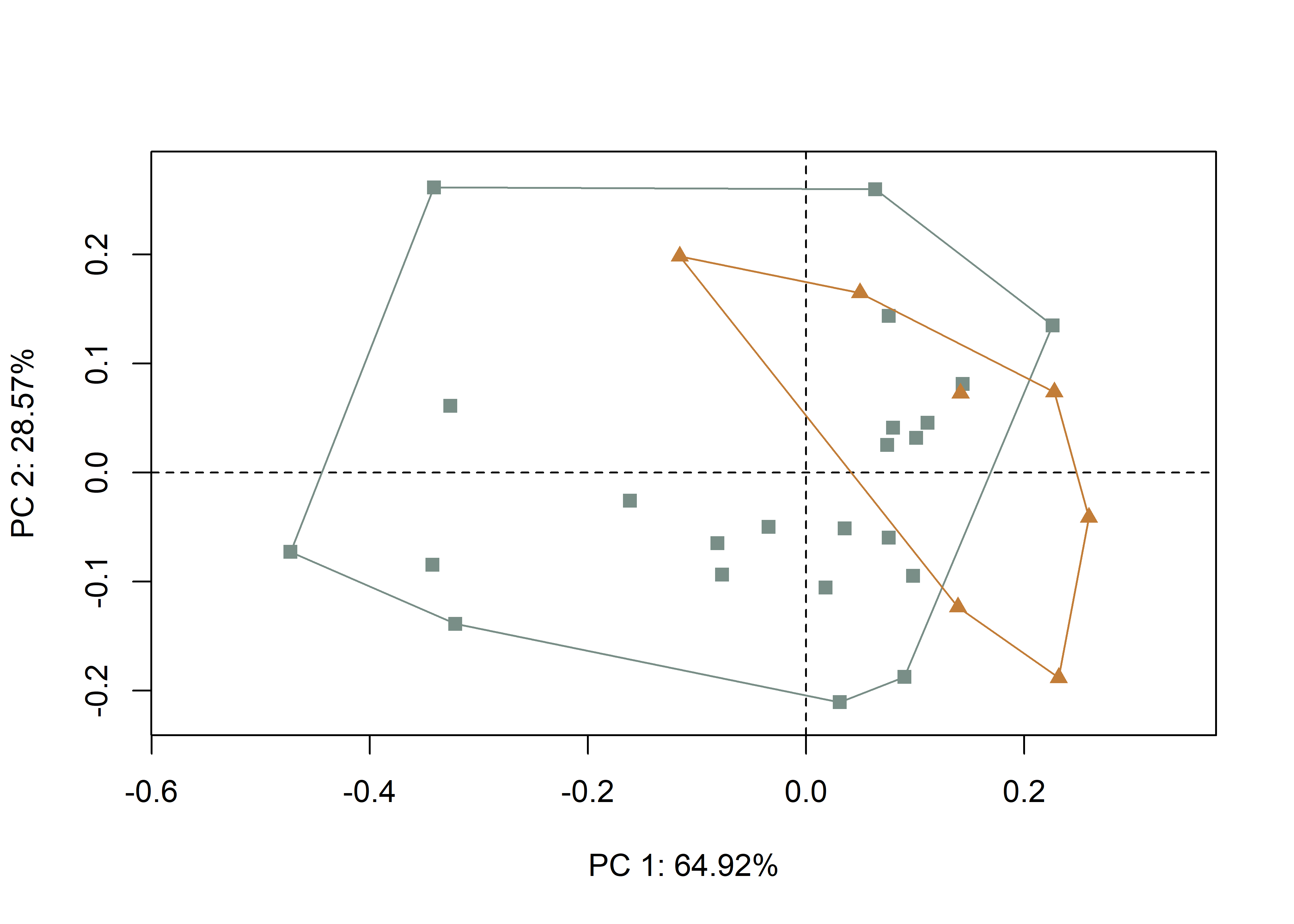

2.4.1 Minima/maxima of PC1/2

# plot x/y maxima/minima
# x - minima
mean.shape <- mshape(Y.gpa$coords)
plotRefToTarget(pca$shapes$shapes.comp1$min, 
                mean.shape)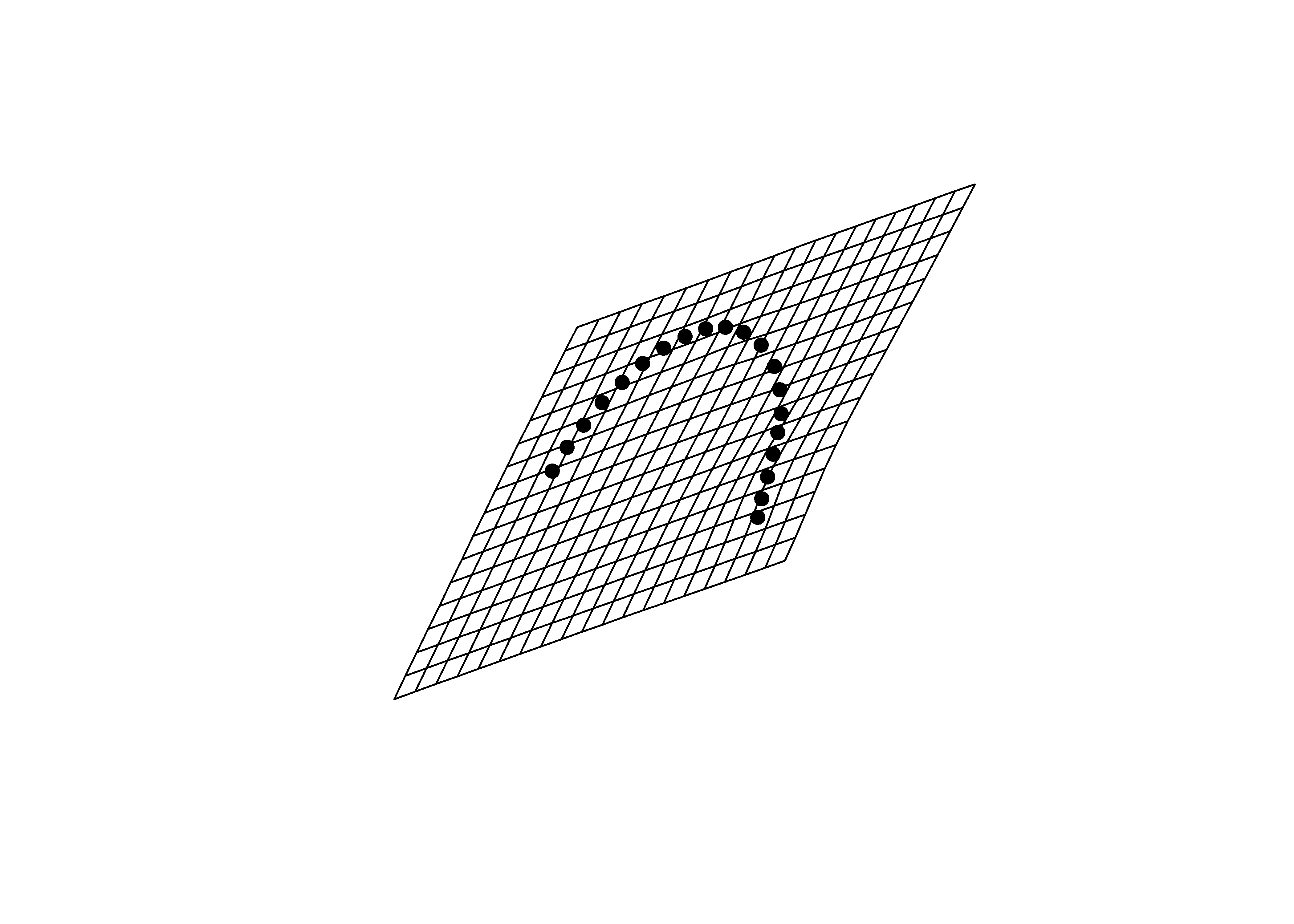

# x - maxima
plotRefToTarget(pca$shapes$shapes.comp1$max, 
                mean.shape)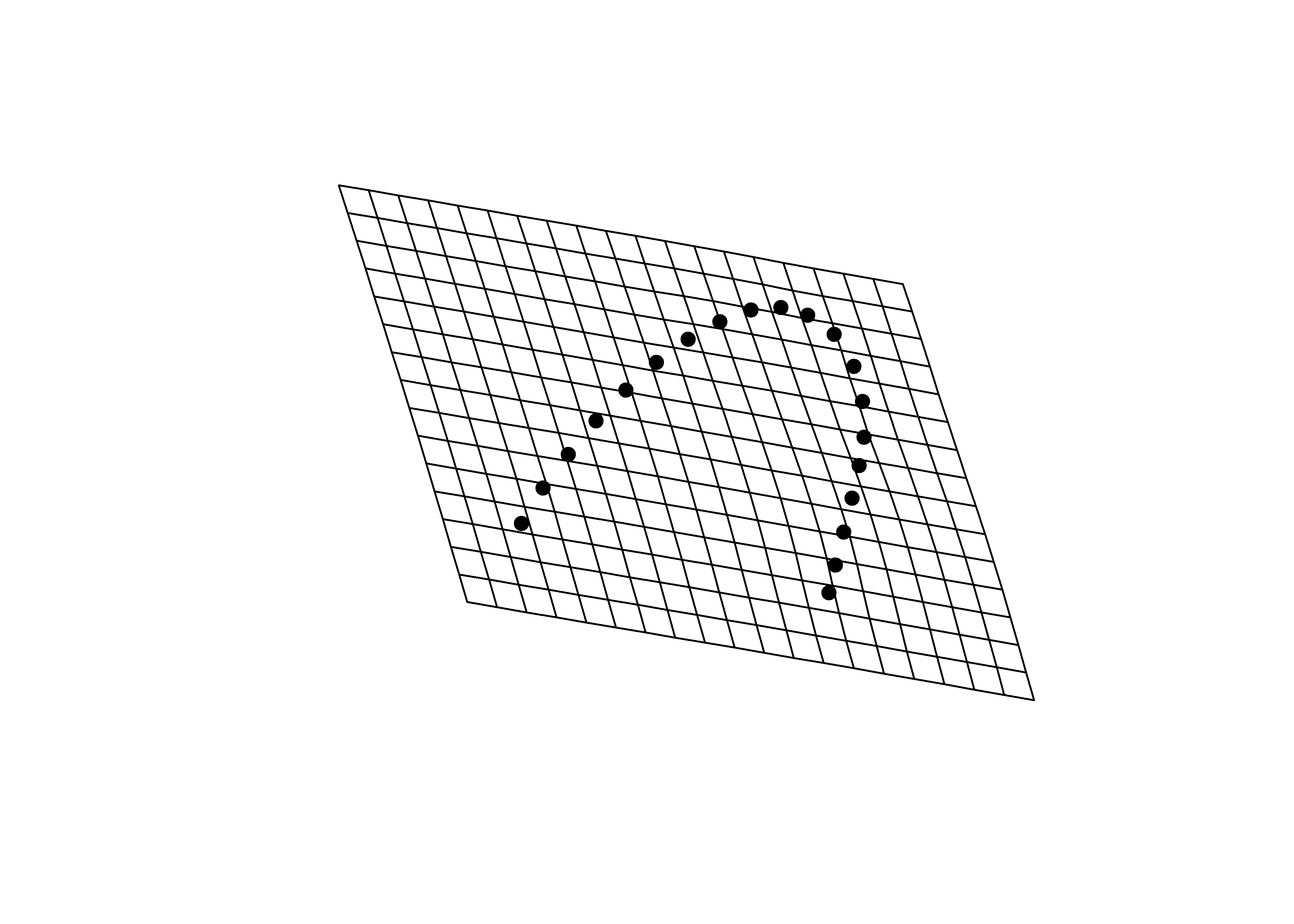

# y - minima
plotRefToTarget(pca$shapes$shapes.comp2$min, 
                mean.shape)

# y - maxima
plotRefToTarget(pca$shapes$shapes.comp2$max, 
                mean.shape)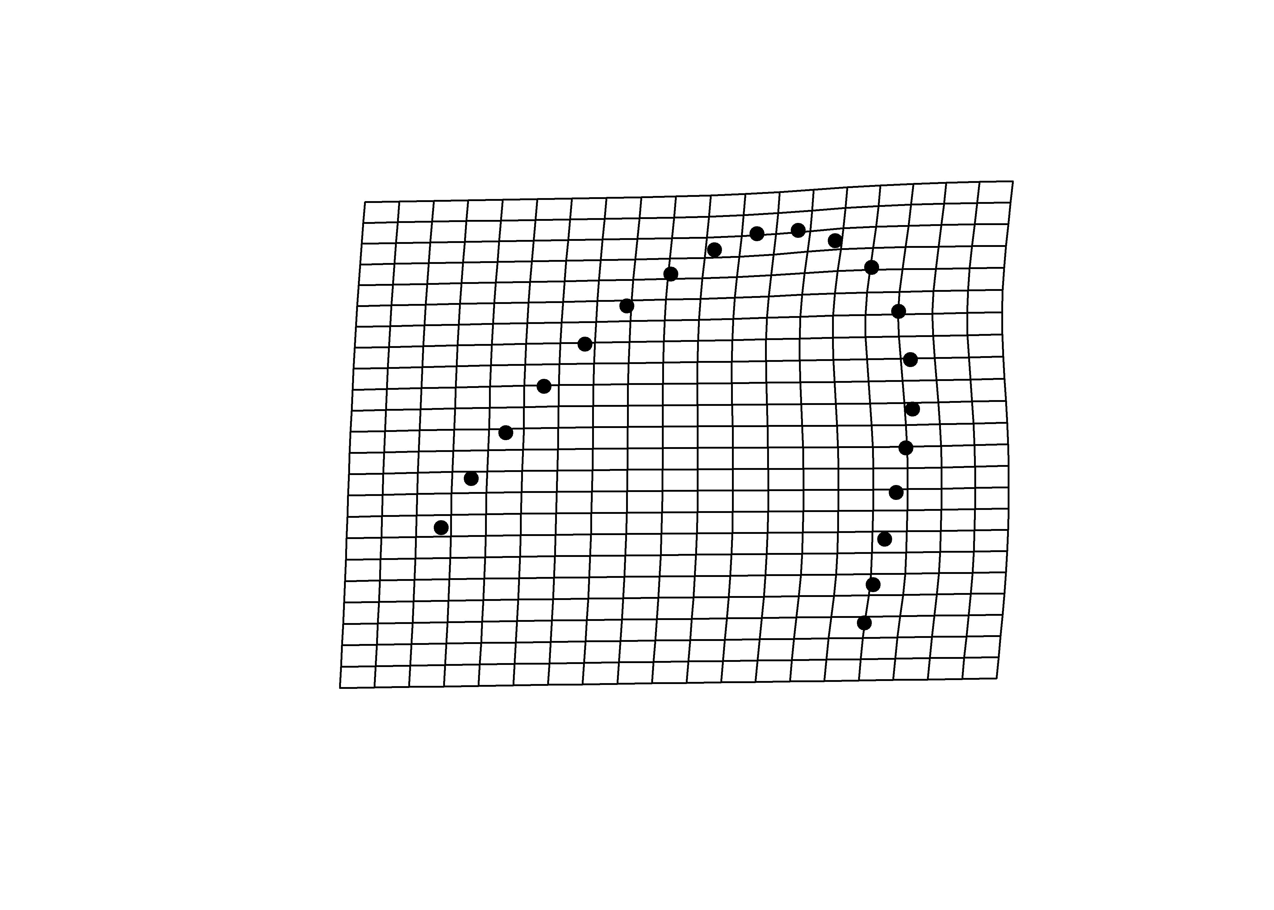

2.5 Procrustes ANOVA: Shape and size

# does shape differ by context?
fit.sh.reg <- procD.lm(shape ~ context,
                       data = gdf,
                       print.progress = FALSE,
                       iter = 9999)

# shape
anova(fit.sh.reg)

## 
## Analysis of Variance, using Residual Randomization
## Permutation procedure: Randomization of null model residuals 
## Number of permutations: 10000 
## Estimation method: Ordinary Least Squares 
## Sums of Squares and Cross-products: Type I 
## Effect sizes (Z) based on F distributions
## 
##           Df      SS       MS     Rsq      F      Z Pr(>F)  
## context    1 0.17877 0.178767 0.10776 3.3816 1.7342 0.0365 *
## Residuals 28 1.48019 0.052864 0.89224                       
## Total     29 1.65896                                        
## ---
## Signif. codes:  0 '***' 0.001 '**' 0.01 '*' 0.05 '.' 0.1 ' ' 1
## 
## Call: procD.lm(f1 = shape ~ context, iter = 9999, data = gdf, print.progress = FALSE)

# does size differ by context?
fit.sz.reg <- procD.lm(size ~ context,
                       data = gdf,
                       print.progress = FALSE,
                       iter = 9999)

# size
anova(fit.sz.reg)

## 
## Analysis of Variance, using Residual Randomization
## Permutation procedure: Randomization of null model residuals 
## Number of permutations: 10000 
## Estimation method: Ordinary Least Squares 
## Sums of Squares and Cross-products: Type I 
## Effect sizes (Z) based on F distributions
## 
##           Df     SS       MS     Rsq      F        Z Pr(>F)
## context    1 0.0275 0.027532 0.00507 0.1426 -0.56399 0.7099
## Residuals 28 5.4054 0.193049 0.99493                       
## Total     29 5.4329                                        
## 
## Call: procD.lm(f1 = size ~ context, iter = 9999, data = gdf, print.progress = FALSE)

2.6 Allometry

# allometry (does shape change with size)
fit.size <- procD.lm(shape ~ size,
                     data = gdf,
                     print.progress = FALSE,
                     iter = 9999)

# allometry
anova(fit.size)

## 
## Analysis of Variance, using Residual Randomization
## Permutation procedure: Randomization of null model residuals 
## Number of permutations: 10000 
## Estimation method: Ordinary Least Squares 
## Sums of Squares and Cross-products: Type I 
## Effect sizes (Z) based on F distributions
## 
##           Df      SS      MS     Rsq      F      Z Pr(>F)  
## size       1 0.16431 0.16431 0.09905 3.0782 1.5966 0.0514 .
## Residuals 28 1.49465 0.05338 0.90095                       
## Total     29 1.65896                                       
## ---
## Signif. codes:  0 '***' 0.001 '**' 0.01 '*' 0.05 '.' 0.1 ' ' 1
## 
## Call: procD.lm(f1 = shape ~ size, iter = 9999, data = gdf, print.progress = FALSE)

2.7 Mean shapes

# subset landmark coordinates to produce mean shapes
new.coords <- coords.subset(A = Y.gpa$coords,
                            group = qdata$context)
names(new.coords)

## [1] "Pit 434"      "Structure 23"

# group shape means
mean <- lapply(new.coords, mshape)

# plot mean shapes
plot(mean$`Pit 434`)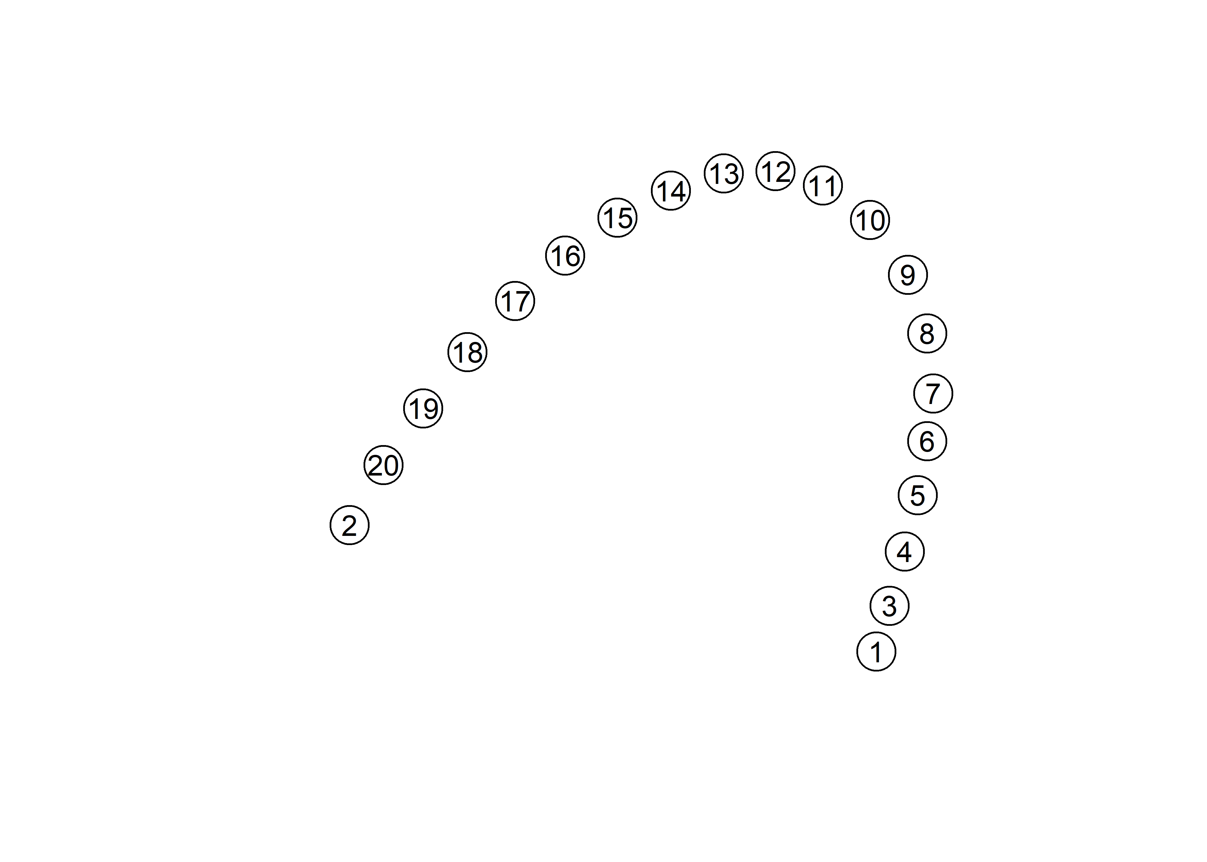

plot(mean$`Structure 23`)

# comparison plots
plotRefToTarget(mean$`Pit 434`,
                mean$`Structure 23`,
                method = "points",
                mag = 1)

References

Adams, Dean C., Michael L. Collyer, Antigoni Kaliontzopoulou, and Emma Sherratt. 2017. “Package ’geomorph’: Geometric Morphometric Analyses of 2D/3D Landmark Data. R package version 3.0.5.” Journal Article. http://geomorphr.github.io/geomorph/.

Adams, Dean C., and Erik Otárola-Castillo. 2013. “geomorph: An R Package for the Collection and Analysis of Geometric Morphometric Shape Data.” Journal Article. Methods in Ecology and Evolution 4 (4): 393–99. https://doi.org/10.1111/2041-210x.12035.

Gower, J. C. 1975. “Generalized Procrustes Analysis.” Journal Article. Psychometrika 40 (1): 33–51. https://doi.org/https://doi.org/10.1007/BF02291478.

Jolliffe, Ian T. 2002. Principal Component Analysis. Book. New York: Springer.

Kendall, David G. 1981. “The Statistics of Shape.” Book Section. In Interpreting Multivariate Data, edited by V. Barnett, 75–80. New York: Wiley.

———. 1984. “Shape Manifolds, Procrustean Metrics, and Complex Projective Spaces.” Journal Article. Bulletin of the London Mathematical Society 16 (2): 81–121. https://doi.org/10.1112/blms/16.2.81.

Klingenberg, Christian Peter. 2013. “Visualizations in Geometric Morphometrics: How to Read and How to Make Graphs Showing Shape Changes.” Journal Article. Hystrix 24 (1): 15–24. https://doi.org/http://dx.doi.org/10.4404/hystrix-24.1-7691.

R Core Development Team,. 2017. R: A Language and Environment for Statistical Computing. Vienna, Austria: R Foundation for Statistical Computing. http://www.R-project.org/.

Rohlf, F. James. 1999. “Shape Statistics: Procrustes Superimpositions and Tangent Spaces.” Journal Article. Journal of Classification 16 (2): 197–223. https://doi.org/10.1007/s003579900054.

Rohlf, F. James, and Dennis Slice. 1990. “Extensions of the Procrustes Method for the Optimal Superimposition of Landmarks.” Journal Article. Systematic Zoology 39 (1): 40–59. https://doi.org/10.2307/2992207.

Sherratt, E., D. J. Gower, C. P. Klingenberg, and M. Wilkinson. 2014. “Evolution of Cranial Shape in Caecilians (Amphibia: Gymnophiona).” Journal Article. Evolutionary Biology 41 (4): 528–45. https://doi.org/https://doi.org/10.1007/s11692-014-9287-2.

Slice, Dennis E. 2001. “Landmark Coordinates Aligned by Procrustes Analysis Do Not Lie in Kendall’s Shape Space.” Journal Article. Systematic Biology 50 (1): 141–49. https://doi.org/10.1080/10635150119110.