Chapter 2 Spatial

# load packages
library(ggplot2)
library(sf)

## Linking to GEOS 3.8.0, GDAL 3.0.4, PROJ 6.3.1

library(rnaturalearth)
library(rnaturalearthdata)
library(ggrepel)
library(ggspatial)
library(maps)
library(tools)

# build map
world <- ne_countries(scale = "medium", 
                      returnclass = "sf")
class(world)

## [1] "sf"         "data.frame"

states <- st_as_sf(map("state", 
                       plot = FALSE, 
                       fill = TRUE))
head(states)

## Simple feature collection with 6 features and 1 field
## geometry type:  MULTIPOLYGON
## dimension:      XY
## bbox:           xmin: -124.3834 ymin: 30.24071 xmax: -71.78015 ymax: 42.04937
## geographic CRS: WGS 84
##            ID                           geom
## 1     alabama MULTIPOLYGON (((-87.46201 3...
## 2     arizona MULTIPOLYGON (((-114.6374 3...
## 3    arkansas MULTIPOLYGON (((-94.05103 3...
## 4  california MULTIPOLYGON (((-120.006 42...
## 5    colorado MULTIPOLYGON (((-102.0552 4...
## 6 connecticut MULTIPOLYGON (((-73.49902 4...

states <- cbind(states, 
                st_coordinates(st_centroid(states)))
states$ID <- toTitleCase(states$ID)
head(states)

## Simple feature collection with 6 features and 3 fields
## geometry type:  MULTIPOLYGON
## dimension:      XY
## bbox:           xmin: -124.3834 ymin: 30.24071 xmax: -71.78015 ymax: 42.04937
## geographic CRS: WGS 84
##            ID          X        Y                           geom
## 1     Alabama  -86.83042 32.80316 MULTIPOLYGON (((-87.46201 3...
## 2     Arizona -111.66786 34.30060 MULTIPOLYGON (((-114.6374 3...
## 3    Arkansas  -92.44013 34.90418 MULTIPOLYGON (((-94.05103 3...
## 4  California -119.60154 37.26901 MULTIPOLYGON (((-120.006 42...
## 5    Colorado -105.55251 38.99797 MULTIPOLYGON (((-102.0552 4...
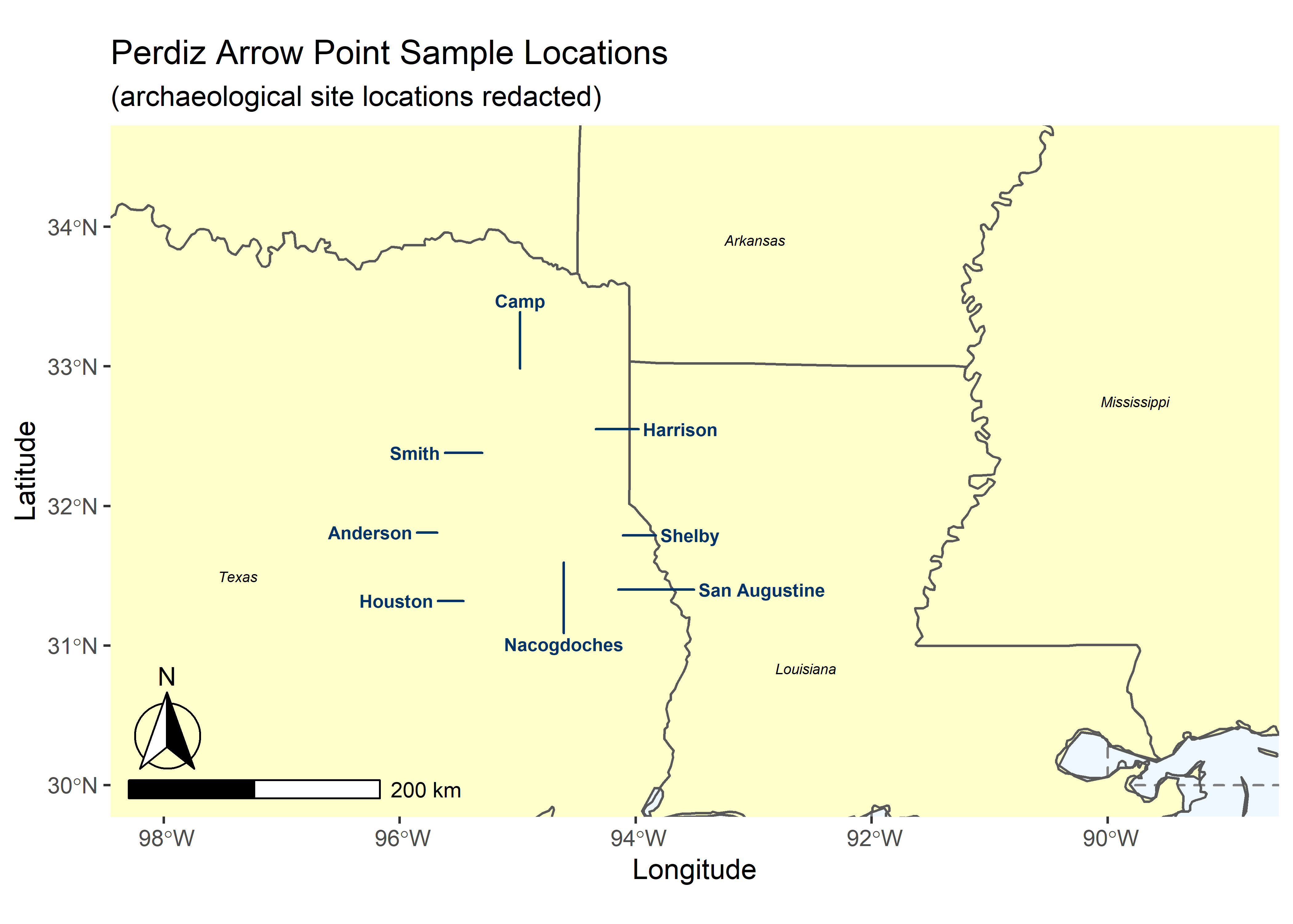
## 6 Connecticut  -72.72598 41.62566 MULTIPOLYGON (((-73.49902 4...

archcentroids <- data.frame(arch = c("Anderson","Camp","Harrison","Houston","Nacogdoches","San Augustine","Smith","Shelby"),
                            lat = c(31.81, 32.97, 32.55, 31.32, 31.61, 31.4, 32.38, 31.79),
                            lng = c(-95.65, -94.98, -94.37, -95.43, -94.61, -94.18, -95.27, -94.14))
states$nudge_x <- -0.55
states$nudge_x[states$ID == "Texas"] <- 2
states$nudge_x[states$ID == "Mississippi"] <- -0.1
states$nudge_y <- -0.01
states$nudge_y[states$ID == "Louisiana"] <- -0.25
states$nudge_y[states$ID == "Arkansas"] <- -1

# plot map
ggplot(data = world) +
  geom_sf(fill = "#FFFFCC") +
  geom_sf(data = states, 
          fill = NA) + 
  geom_text(data = states, 
            aes(X, Y, label = ID), 
            nudge_x = states$nudge_x, 
            nudge_y = states$nudge_y, 
            fontface = "italic", size = 2) +
  geom_text_repel(data = archcentroids, aes(x = lng, y = lat, label = arch), 
                  fontface = "bold", 
                  nudge_x = c(-0.6,0,0.75,-0.6,0,1.25,-0.6,0.6), 
                  nudge_y = c(0,0.5,0,0,-0.6,0,0,0), 
                  color = "#003366", 
                  size = 2.5) +
  coord_sf(xlim = c(-98, -89), 
           ylim = c(30, 34.5), 
           expand = TRUE) +
  ggtitle("Perdiz Arrow Point Sample Locations", 
          subtitle = "(archaeological site locations redacted)") +
  annotation_scale(location = "bl", 
                   width_hint = 0.3) +
  annotation_north_arrow(location = "bl", 
                         which_north = "true", 
                         pad_x = unit(0.01, "in"), 
                         pad_y = unit(0.2, "in"),
                         style = north_arrow_fancy_orienteering) +
  theme(panel.grid.major = element_line(color = gray(0.5), 
                                        linetype = "dashed", 
                                        size = 0.5), 
        panel.background = element_rect(fill = "aliceblue")) +
  labs(x = "Longitude", y = "Latitude")