Chapter 4 Experimental sample - analysis
The inc field in the qdataEX file relates to two primary differences in shape. One U-shaped, and the other V-shaped. The inc2 field in the qdataEX file relates to the differences in shape that were noted when reviewing general incision morphology. Some were U-shaped and narrow, others U-shaped and wide (twice as wide as they are deep), and the remainder were V-shaped.
The narrow and wide U-shaped incisions were made by different tools; however, it is not at all difficult to imagine a scenario where both of the U-shaped incisions could also have been produced with two different sides of the same tool. It is thus necessary to use abundant caution when interpreting potential tool shape, or the number of tools employed in the application of incisions. To avoid confounding the issue, the tip of each of the tools used to generate the incision is referred to as a bit in the remainder of this document. Tools may have multiple bits, but each bit is capable of generating different incision profiles.
4.1 Load packages + data
# download analysis packages
#devtools::install_github("geomorphR/geomorph", ref = "Stable", build_vignettes = TRUE)
#devtools::install_github("mlcollyer/RRPP")

# load
library(here)
## here() starts at C:/Users/selde/Desktop/github/incisionlibrary(geomorph)## Loading required package: RRPP## Loading required package: rgl## Loading required package: Matrixlibrary(tidyverse)## ── Attaching packages
## ───────────────────────────────────────────────────
## tidyverse 1.3.2 ──## ✔ tibble 3.1.8 ✔ dplyr 1.0.10
## ✔ tidyr 1.2.1 ✔ stringr 1.4.1
## ✔ readr 2.1.3 ✔ forcats 0.5.2
## ✔ purrr 0.3.5
## ── Conflicts ────────────────────────────────────────────────────── tidyverse_conflicts() ──
## ✖ tidyr::expand() masks Matrix::expand()
## ✖ dplyr::filter() masks stats::filter()
## ✖ dplyr::lag() masks stats::lag()
## ✖ tidyr::pack() masks Matrix::pack()
## ✖ tidyr::unpack() masks Matrix::unpack()library(wesanderson)
# Read shape data
source('readmulti.csv.R')
setwd("./dataEX")
filelist <- list.files(pattern = ".csv")
coords <- readmulti.csv(filelist)
setwd("../")
# read qualitative data
qdata <- read.csv("qdataEX.csv",
header = TRUE,
row.names = 1)
qdata <- qdata[match(dimnames(coords)[[3]],rownames(qdata)),]
# print qdata
knitr::kable(qdata,
align = "cc",
caption = "Attributes included in qdata.")| incision | inc2 | |
|---|---|---|
| ex-tile2 | U | Un |
| ex-tile3a | U | Uw |
| ex-tile3b | V | V |
| ex-tile4a | U | Un |
| ex-tile4b | V | V |
| ex-tile5a | V | V |
| ex-tile5b | U | Un |
| ex-tile6a | U | Un |
| ex-tile6b | V | V |
| ex-tile7a | U | Uw |
| ex-tile7b | V | V |
| ex-tile8a | U | Uw |
| ex-tile8b | V | V |
4.2 Generalised Procrustes Analysis
Y.gpa <- gpagen(coords,
                PrinAxes = TRUE,
                ProcD = TRUE,
                Proj = TRUE,
                print.progress = FALSE)

# 3D GPA plot
knitr::include_graphics('images/gpa3dEX.png')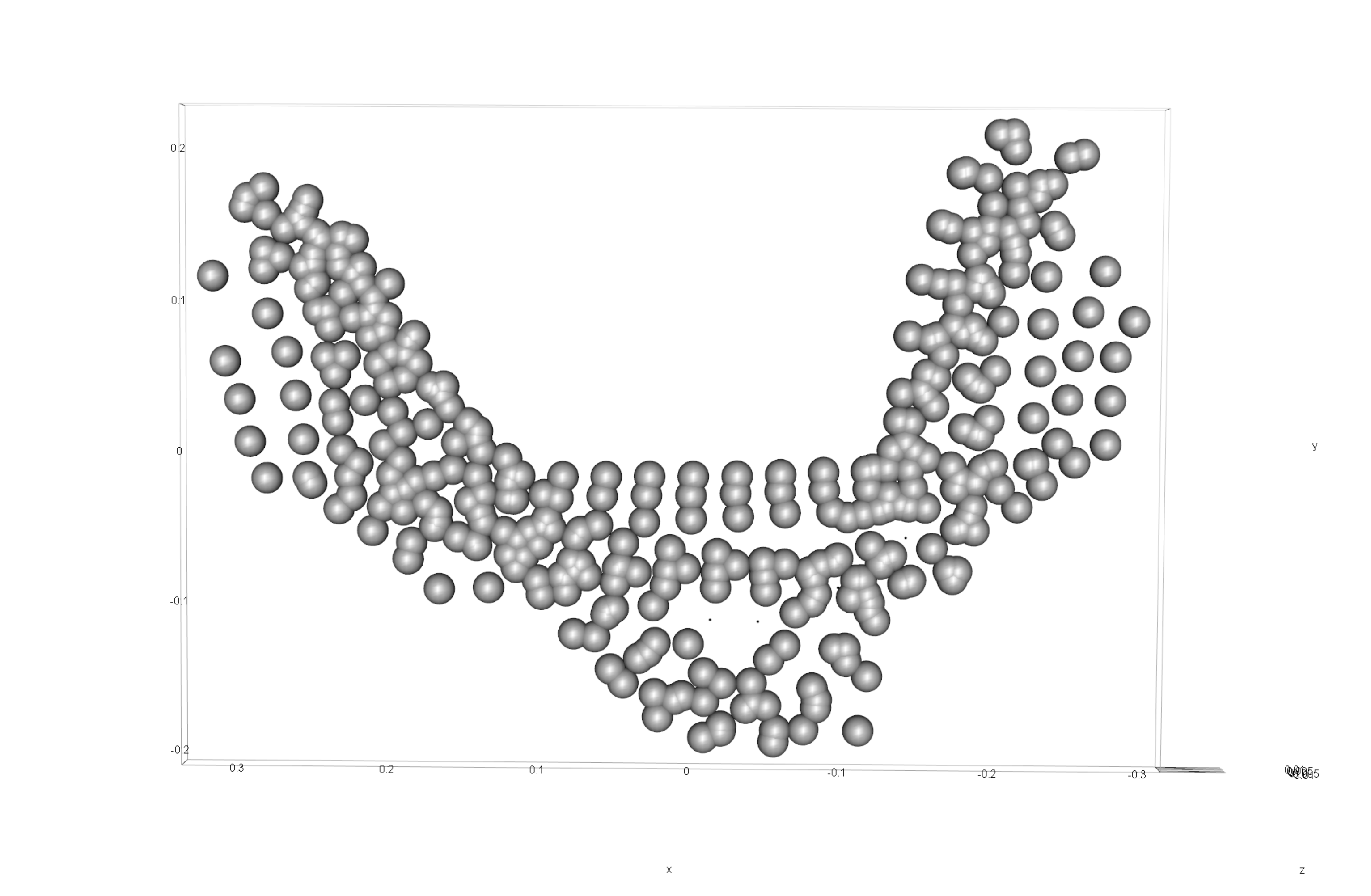
Figure 4.1: Results of generalised Procrustes analysis.
# geomorph data frame
gdf <- geomorph.data.frame(shape = Y.gpa$coords,
                           size = Y.gpa$Csize,
                           inc = qdata$incision,
                           inc2 = qdata$inc2)
# add centroid size to qdata
qdata$csz <- Y.gpa$Csize
# attributes for boxplots
csz <- qdata$csz
inc <- qdata$incision
inc2 <- qdata$inc2
# print qdata + centroid size
knitr::kable(qdata,
align = "ccc",
caption = "Attributes included in qdata.")| incision | inc2 | csz | |
|---|---|---|---|
| ex-tile2 | U | Un | 7.457707 |
| ex-tile3a | U | Uw | 13.962369 |
| ex-tile3b | V | V | 6.057672 |
| ex-tile4a | U | Un | 6.709478 |
| ex-tile4b | V | V | 4.636639 |
| ex-tile5a | V | V | 4.817187 |
| ex-tile5b | U | Un | 7.124874 |
| ex-tile6a | U | Un | 10.150058 |
| ex-tile6b | V | V | 10.518014 |
| ex-tile7a | U | Uw | 15.273933 |
| ex-tile7b | V | V | 10.073934 |
| ex-tile8a | U | Uw | 18.107928 |
| ex-tile8b | V | V | 10.002956 |
# boxplot of incision (centroid) size by profile type (inc)
csz.inc.ex <- ggplot(qdata, aes(x = inc, y = csz, color = inc)) +
  geom_boxplot() +
  geom_dotplot(binaxis = 'y', stackdir = 'center', dotsize = 0.3) +
  scale_color_manual(values = wes_palette("Moonrise2")) +
  theme(legend.position = "none") +
  labs(x = 'Incision', y = 'Centroid Size')

#render plot
csz.inc.ex
## Bin width defaults to 1/30 of the range of the data. Pick better value with `binwidth`.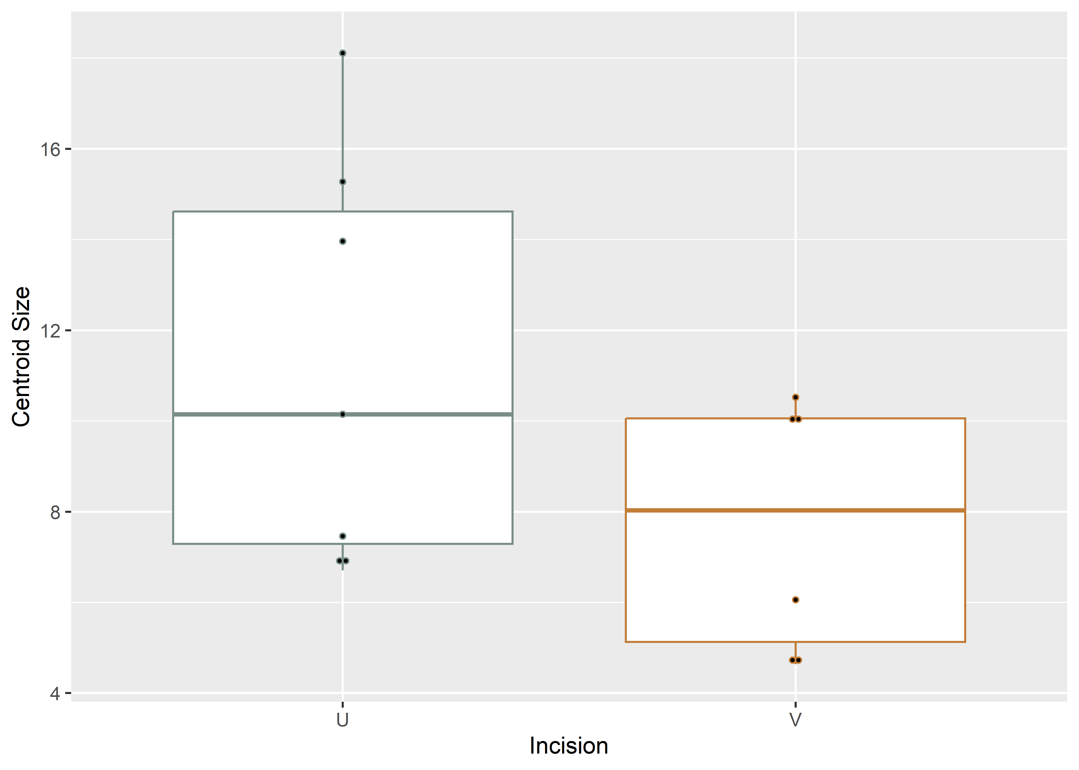
Figure 4.2: Boxplot of experimental incision profile types (U-shaped and V-shaped).
# boxplot of incision (centroid) size by profile type (inc2)
csz.inc2.ex <- ggplot(qdata, aes(x = inc2, y = csz, color = inc2)) +
  geom_boxplot() +
  geom_dotplot(binaxis = 'y', stackdir = 'center', dotsize = 0.3) +
  scale_color_manual(values = wes_palette("Moonrise2")) +
  theme(legend.position = "none") +
  labs(x = 'Incision', y = 'Centroid Size')

#render plot
csz.inc2.ex
## Bin width defaults to 1/30 of the range of the data. Pick better value with `binwidth`.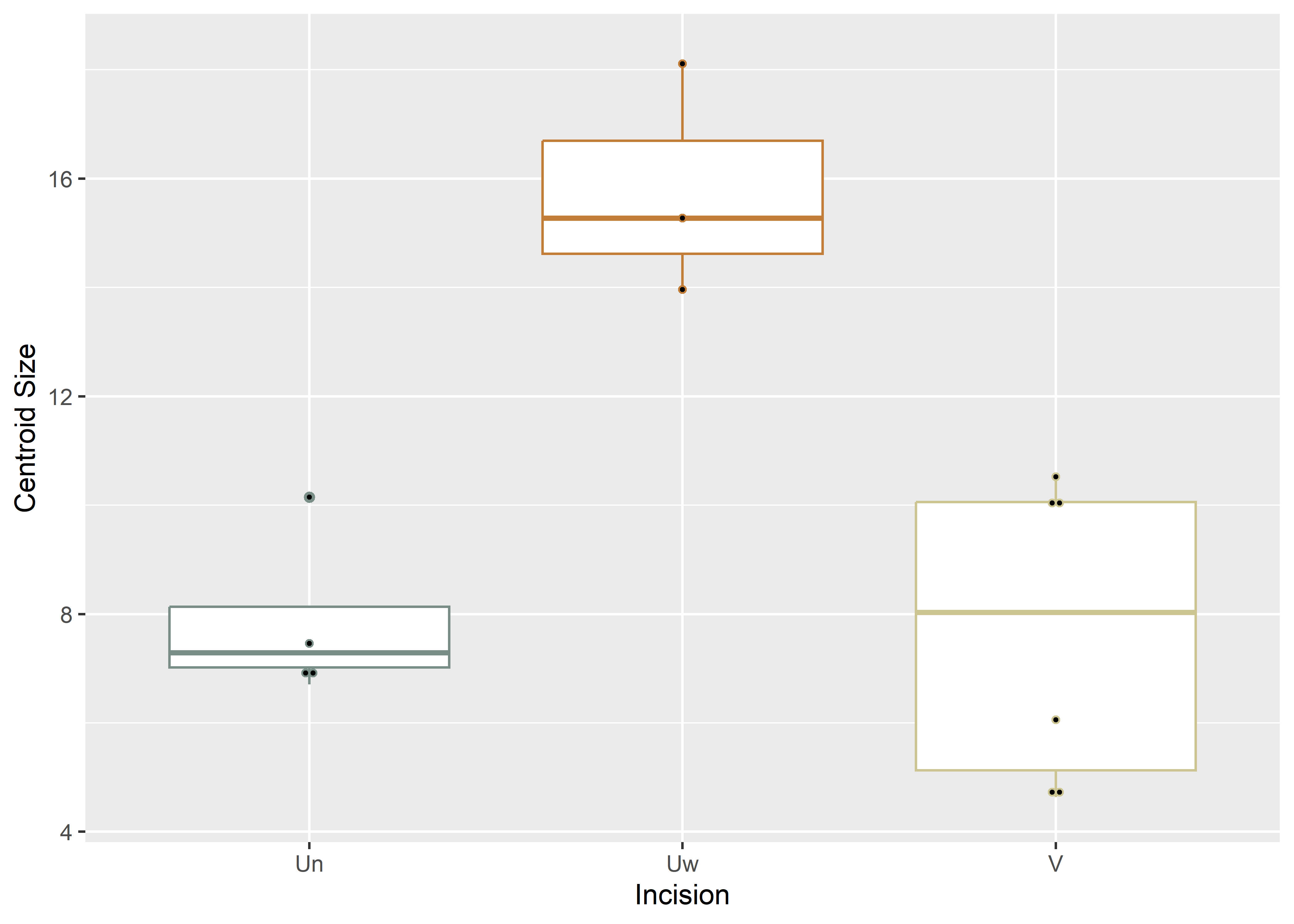
Figure 4.3: Boxplot of experimental incision profile types (U-narrow, U-Wide, and V).
4.3 Principal Components Analysis
# principal components analysis
pca <- gm.prcomp(Y.gpa$coords)
summary(pca)
##
## Ordination type: Principal Component Analysis
## Centering by OLS mean
## Orthogonal projection of OLS residuals
## Number of observations: 13
## Number of vectors 12
##
## Importance of Components:
## Comp1 Comp2 Comp3 Comp4 Comp5
## Eigenvalues 0.0441045 0.005014108 0.003398275 0.0003353507 0.0002822004
## Proportion of Variance 0.8226607 0.093525803 0.063386441 0.0062551403 0.0052637514
## Cumulative Proportion 0.8226607 0.916186472 0.979572913 0.9858280536 0.9910918051
## Comp6 Comp7 Comp8 Comp9 Comp10
## Eigenvalues 0.0001809061 0.0001525644 7.081347e-05 3.658645e-05 2.060166e-05
## Proportion of Variance 0.0033743561 0.0028457127 1.320850e-03 6.824299e-04 3.842732e-04
## Cumulative Proportion 0.9944661611 0.9973118738 9.986327e-01 9.993152e-01 9.996994e-01
## Comp11 Comp12
## Eigenvalues 1.050025e-05 5.614060e-06
## Proportion of Variance 1.958562e-04 1.047164e-04
## Cumulative Proportion 9.998953e-01 1.000000e+00# set plot parameters
pch.gps.1 <- c(15,17)[as.factor(inc)]
col.gps.1 <- wes_palette("Moonrise2")[as.factor(inc)]
col.hull.1 <- c("#798E87","#C27D38")
# plotPCAbyinc2
pc.plot.1 <- plot(pca,asp = 1,
pch = pch.gps.1,
col = col.gps.1)
shapeHulls(pc.plot.1,
groups = inc,
group.cols = col.hull.1)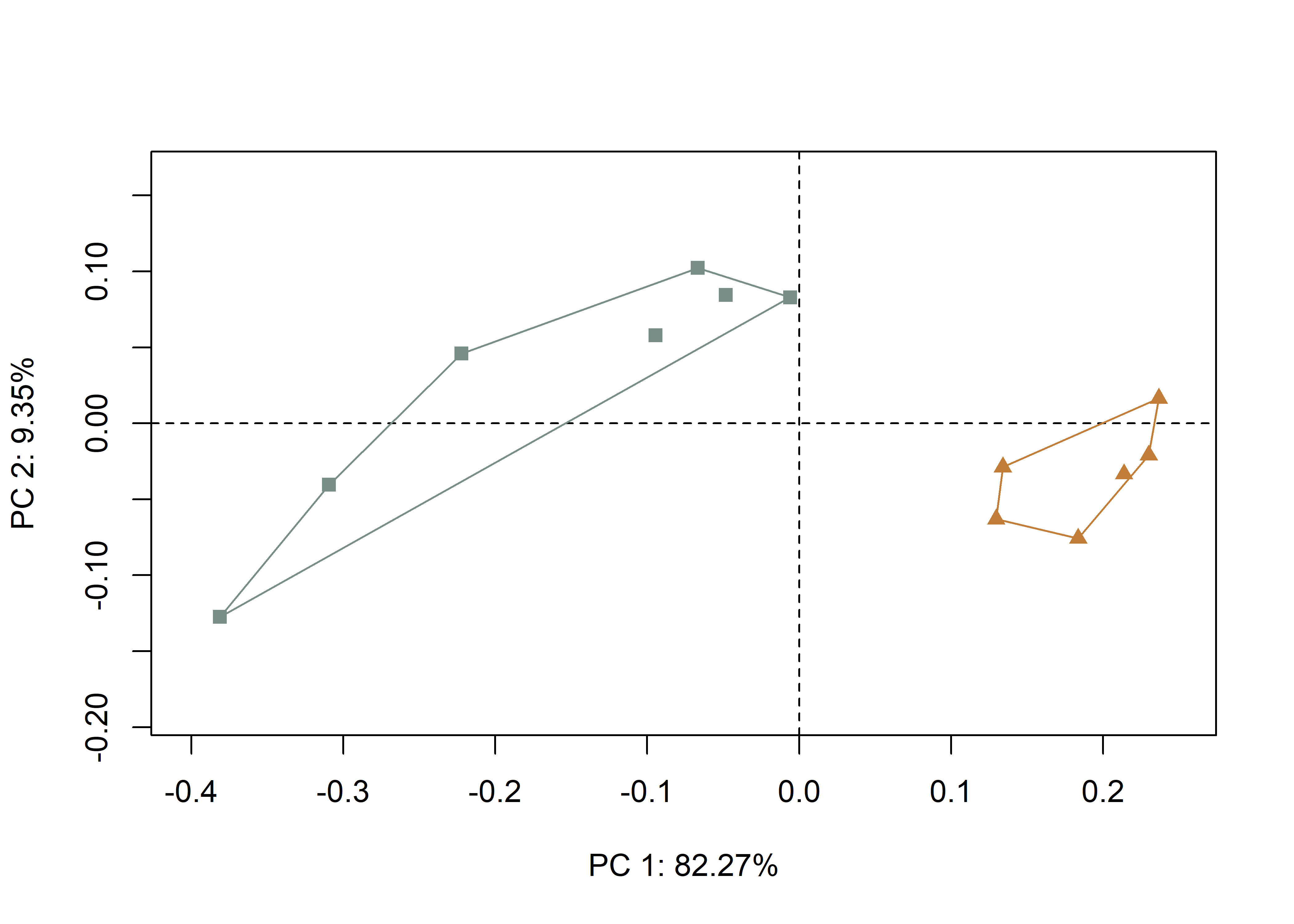
Figure 4.4: Plot of PC1 and PC2 for U- (gray) and V-shaped (orange) incisions.
# set plot parameters
pch.gps.2 <- c(15,17,19)[as.factor(inc2)]
col.gps.2 <- wes_palette("Moonrise2")[as.factor(inc2)]
col.hull.2 <- c("#798E87","#C27D38","#CCC591")

# plotPCAbyinc2
pc.plot.2 <- plot(pca,asp = 1,
            pch = pch.gps.2,
            col = col.gps.2)
            shapeHulls(pc.plot.2,
                       groups = inc2,
                       group.cols = col.hull.2)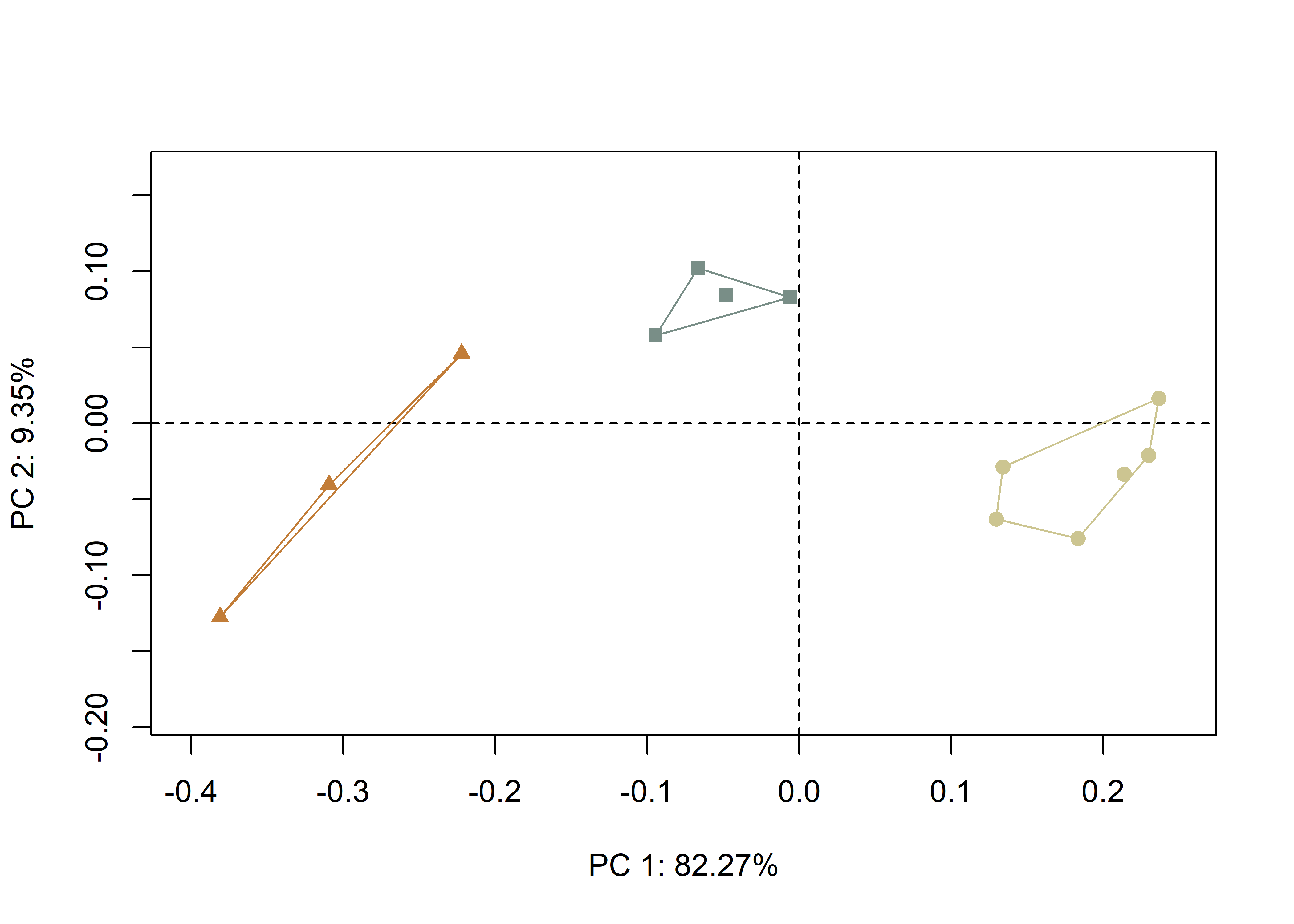
Figure 4.5: Plot of PC1 and PC2; tan circles, V-shaped incisions; gray squares, U-narrow incisions; and orange triangles, U-wide incisions.
4.4 Define models
# allometry
fit.size <- procD.lm(shape ~ size,
                     data = gdf,
                     print.progress = FALSE,
                     iter = 9999)

# allometry - common allometry, different means -> inc
fit.sz.cinc <- procD.lm(shape ~ size + inc,
                        data = gdf,
                        print.progress = FALSE,
                        iter = 9999)

# allometry - unique allometries -> inc
fit.sz.uinc <- procD.lm(shape ~ size * inc,
                        data = gdf,
                        print.progress = FALSE,
                        iter = 9999)

# allometry - common allometry, different means -> inc2
fit.sz.cinc2 <- procD.lm(shape ~ size + inc2,
                         data = gdf,
                         print.progress = FALSE,
                         iter = 9999)

# allometry - unique allometries -> inc2
fit.sz.uinc2 <- procD.lm(shape ~ size * inc2,
                         data = gdf,
                         print.progress = FALSE,
                         iter = 9999)

# size as a function of group
fit.sizeinc <- procD.lm(size ~ inc,
                        data = gdf,
                        print.progress = FALSE,
                        iter = 9999)

fit.sizeinc2 <- procD.lm(size ~ inc2,
                         data = gdf,
                         print.progress = FALSE,
                         iter = 9999)

# shape as a function of group
fit.shapeinc <- procD.lm(shape ~ inc,
                         data = gdf,
                         print.progress = FALSE,
                         iter = 9999)

fit.shapeinc2 <- procD.lm(shape ~ inc2,
                          data = gdf,
                          print.progress = FALSE,
                          iter = 9999)
4.5 Allometry
# allometry - does shape change with size?
anova(fit.size)
##
## Analysis of Variance, using Residual Randomization
## Permutation procedure: Randomization of null model residuals
## Number of permutations: 10000
## Estimation method: Ordinary Least Squares
## Sums of Squares and Cross-products: Type I
## Effect sizes (Z) based on F distributions
##
## Df SS MS Rsq F Z Pr(>F)
## size 1 0.28340 0.283400 0.44051 8.6608 2.3784 0.0052 **
## Residuals 11 0.35994 0.032722 0.55949
## Total 12 0.64334
## ---
## Signif. codes: 0 '***' 0.001 '**' 0.01 '*' 0.05 '.' 0.1 ' ' 1
##
## Call: procD.lm(f1 = shape ~ size, iter = 9999, data = gdf, print.progress = FALSE)4.5.1 Common allometry
# inc
anova(fit.sz.cinc) # common allometry (inc)
##
## Analysis of Variance, using Residual Randomization
## Permutation procedure: Randomization of null model residuals
## Number of permutations: 10000
## Estimation method: Ordinary Least Squares
## Sums of Squares and Cross-products: Type I
## Effect sizes (Z) based on F distributions
##
## Df SS MS Rsq F Z Pr(>F)
## size 1 0.28340 0.283400 0.44051 21.032 3.1698 1e-04 ***
## inc 1 0.22519 0.225195 0.35004 16.712 3.1780 1e-04 ***
## Residuals 10 0.13475 0.013475 0.20945
## Total 12 0.64334
## ---
## Signif. codes: 0 '***' 0.001 '**' 0.01 '*' 0.05 '.' 0.1 ' ' 1
##
## Call: procD.lm(f1 = shape ~ size + inc, iter = 9999, data = gdf, print.progress = FALSE)# inc2
anova(fit.sz.cinc2) # common allometry (inc2)##
## Analysis of Variance, using Residual Randomization
## Permutation procedure: Randomization of null model residuals
## Number of permutations: 10000
## Estimation method: Ordinary Least Squares
## Sums of Squares and Cross-products: Type I
## Effect sizes (Z) based on F distributions
##
## Df SS MS Rsq F Z Pr(>F)
## size 1 0.28340 0.283400 0.44051 26.361 3.3157 1e-04 ***
## inc2 2 0.26319 0.131593 0.40909 12.240 3.2927 3e-04 ***
## Residuals 9 0.09676 0.010751 0.15040
## Total 12 0.64334
## ---
## Signif. codes: 0 '***' 0.001 '**' 0.01 '*' 0.05 '.' 0.1 ' ' 1
##
## Call: procD.lm(f1 = shape ~ size + inc2, iter = 9999, data = gdf, print.progress = FALSE)# allometry plots
# regscore (Drake and Klingenberg 2008)
plot(fit.size,
type = "regression",
reg.type = "RegScore",
predictor = log(gdf$size),
pch = pch.gps.1,
col = col.gps.1)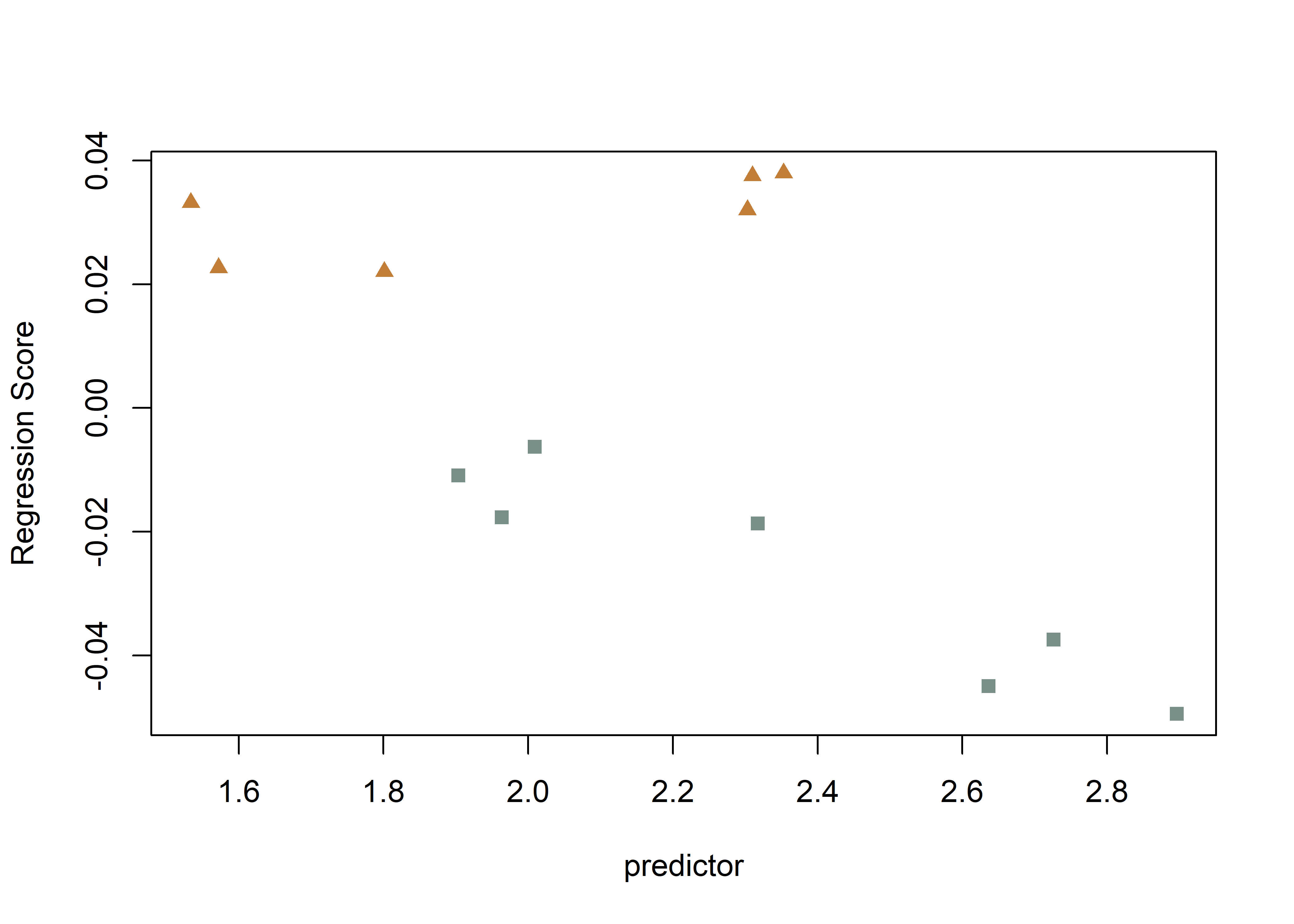
plot(fit.size, type = "regression",
     reg.type = "RegScore",
     predictor = log(gdf$size),
     pch = pch.gps.2,
     col = col.gps.2)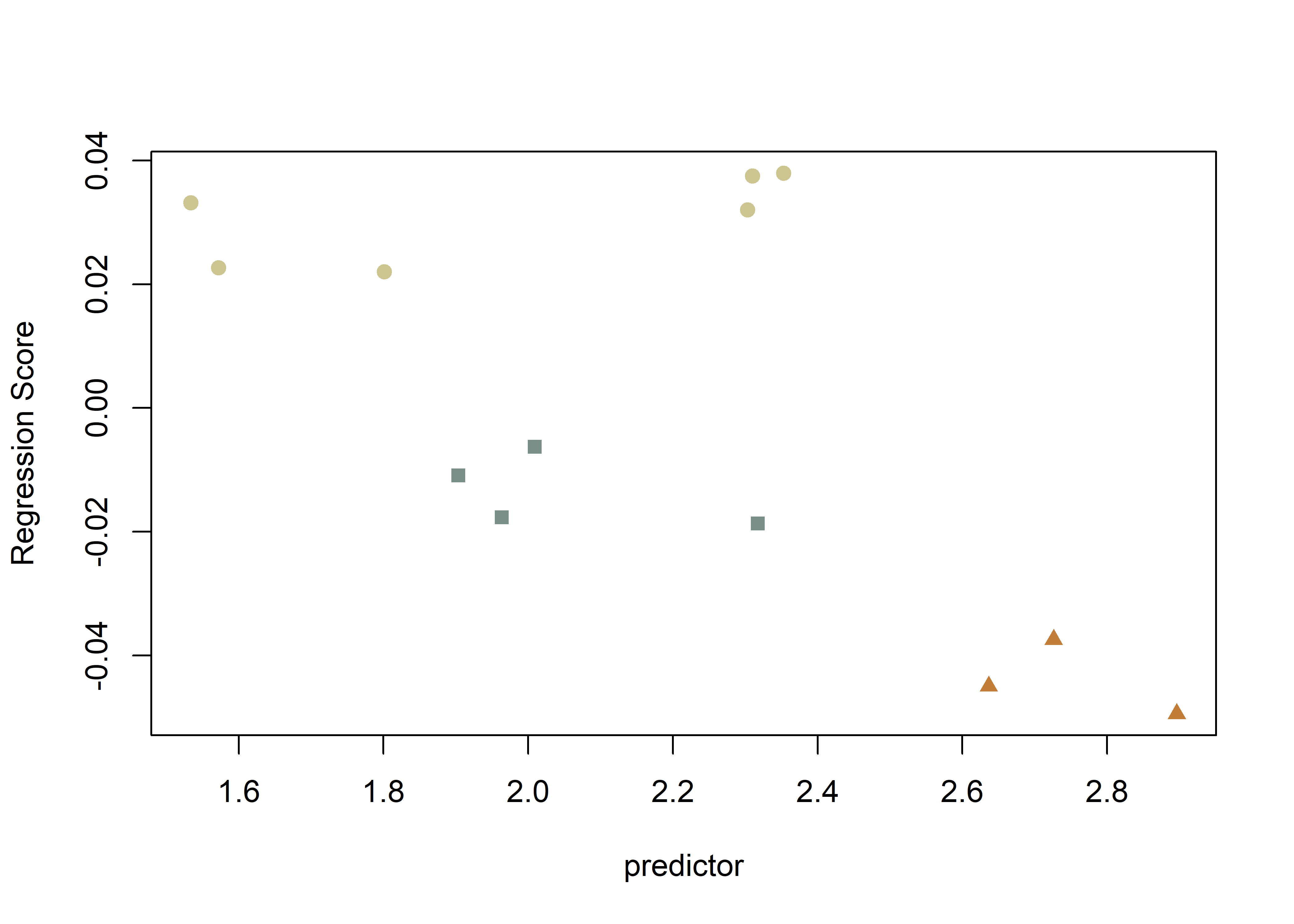
# common allometric component (Mitteroecker 2004)
plotAllometry(fit.size,
              size = gdf$size,
              logsz = TRUE,
              method = "CAC",
              pch = pch.gps.1,
              col = col.gps.1)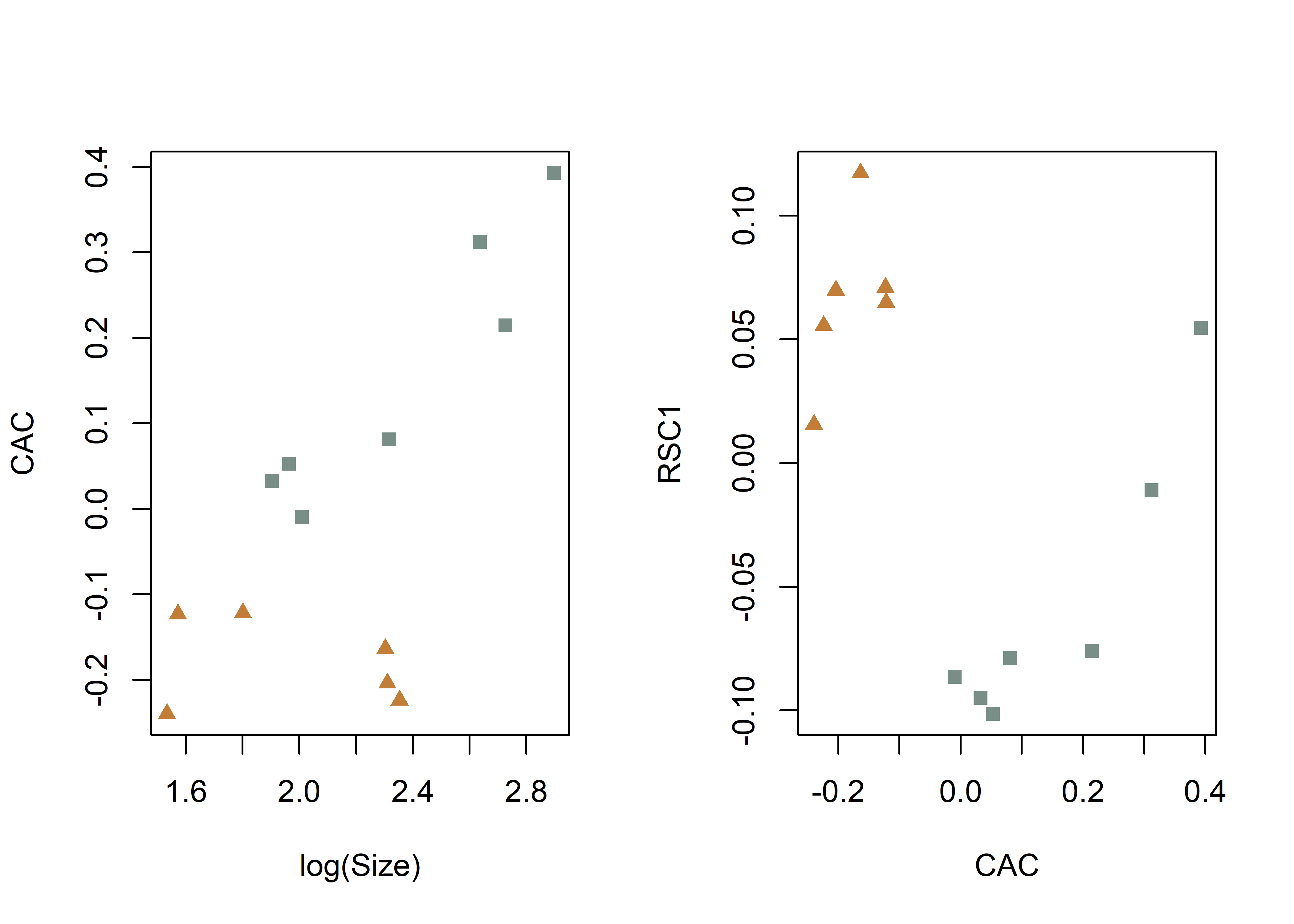
plotAllometry(fit.size,
              size = gdf$size,
              logsz = TRUE,
              method = "CAC",
              pch = pch.gps.2,
              col = col.gps.2)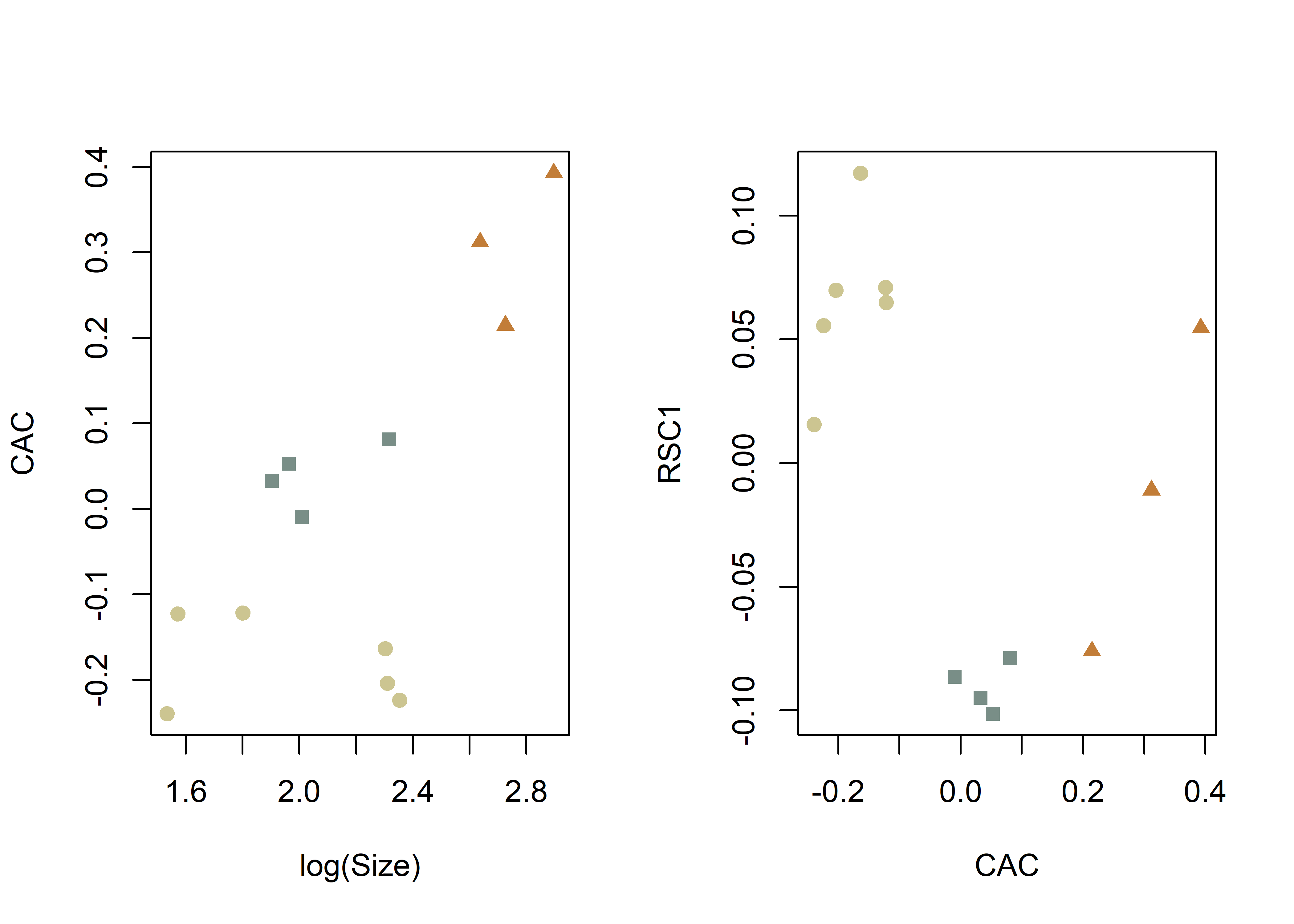
# size-shape pca (Mitteroecker 2004)
plotAllometry(fit.size,
              size = gdf$size,
              logsz = TRUE,
              method = "size.shape",
              pch = pch.gps.1,
              col = col.gps.1)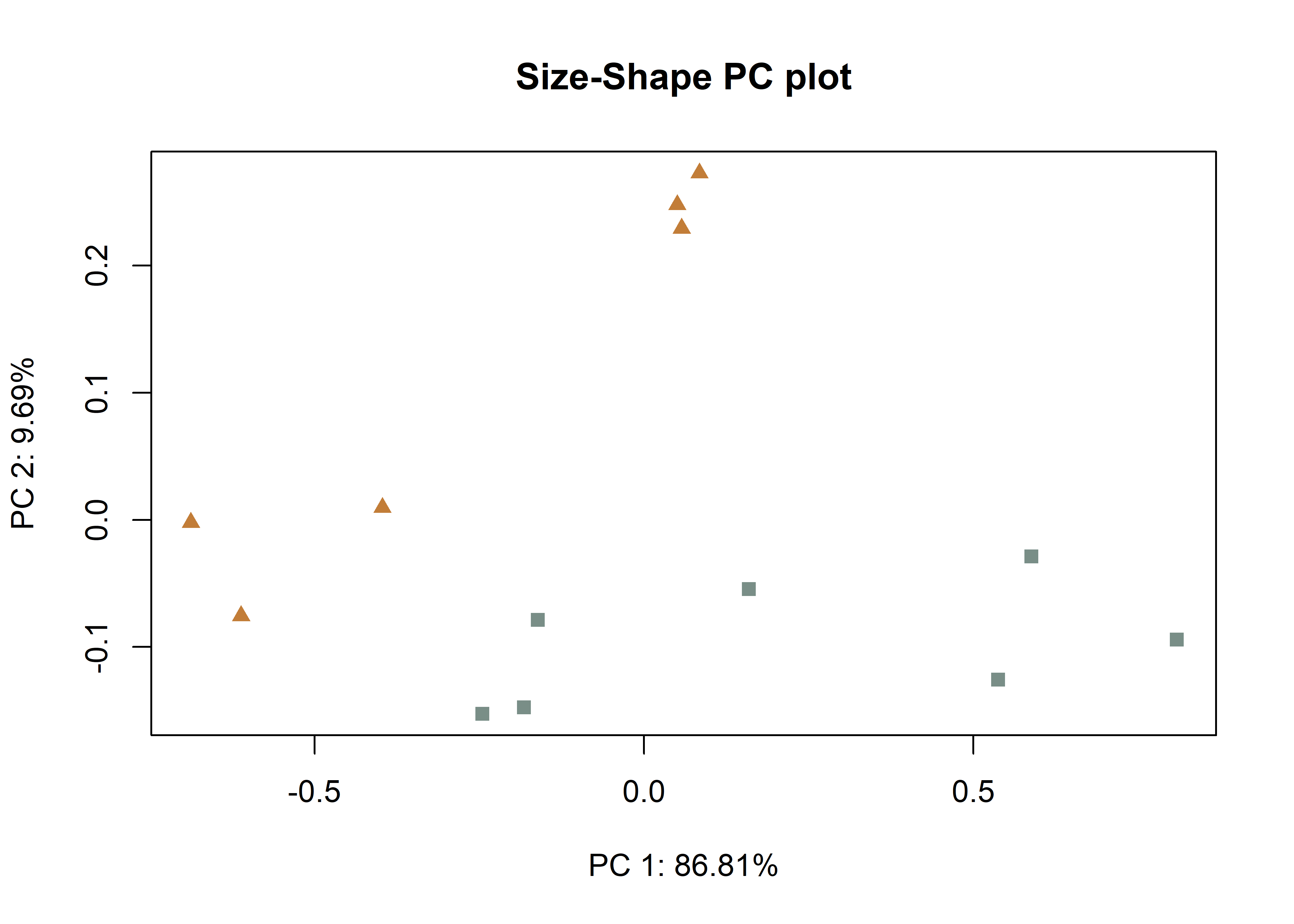
plotAllometry(fit.size,
              size = gdf$size,
              logsz = TRUE,
              method = "size.shape",
              pch = pch.gps.2,
              col = col.gps.2)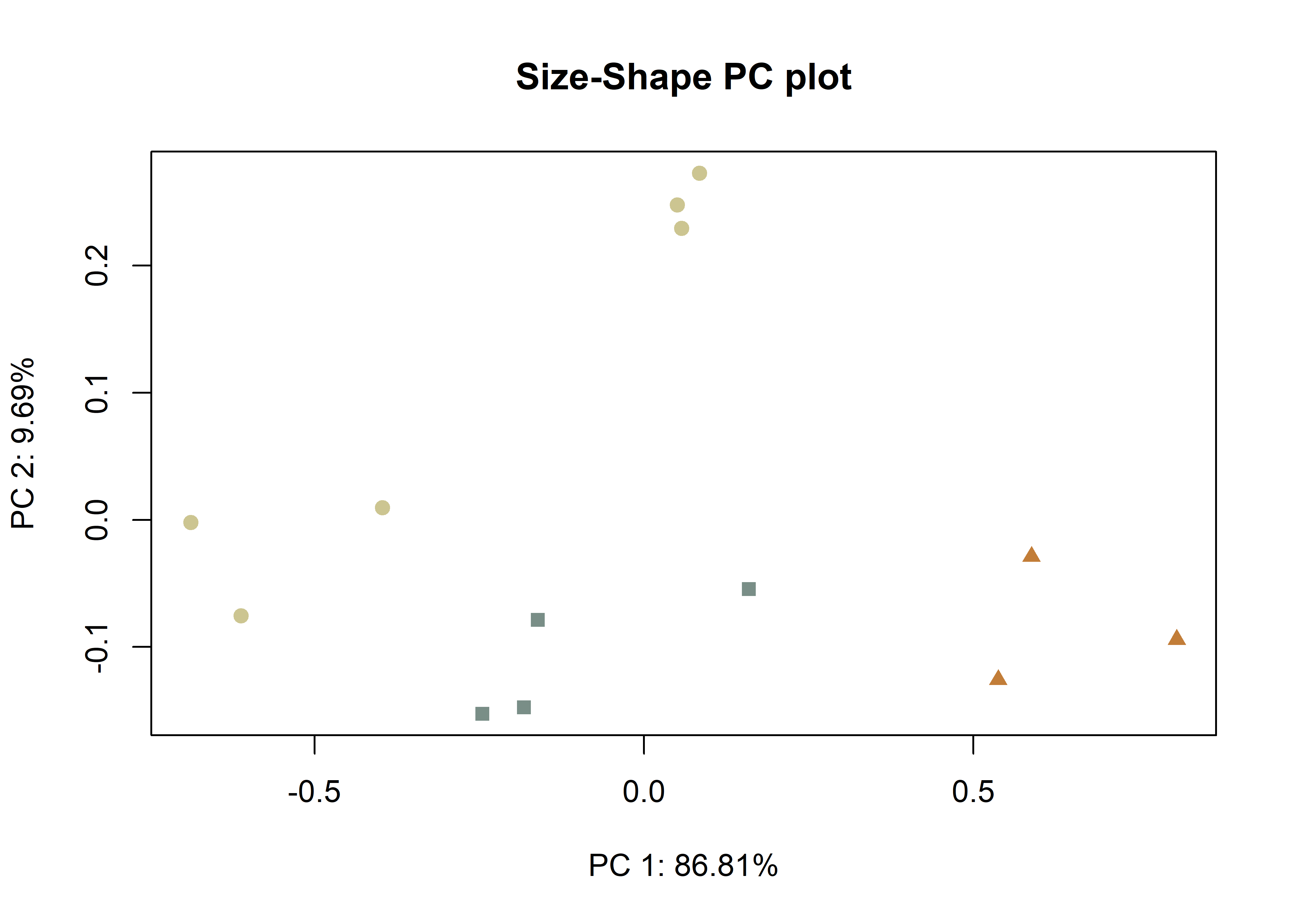
4.5.2 Unique allometry
# inc
anova(fit.sz.uinc) # unique allometry (inc)
##
## Analysis of Variance, using Residual Randomization
## Permutation procedure: Randomization of null model residuals
## Number of permutations: 10000
## Estimation method: Ordinary Least Squares
## Sums of Squares and Cross-products: Type I
## Effect sizes (Z) based on F distributions
##
## Df SS MS Rsq F Z Pr(>F)
## size 1 0.28340 0.283400 0.44051 29.8384 3.4401 1e-04 ***
## inc 1 0.22519 0.225195 0.35004 23.7101 3.4595 1e-04 ***
## size:inc 1 0.04927 0.049269 0.07658 5.1874 2.2701 0.0104 *
## Residuals 9 0.08548 0.009498 0.13287
## Total 12 0.64334
## ---
## Signif. codes: 0 '***' 0.001 '**' 0.01 '*' 0.05 '.' 0.1 ' ' 1
##
## Call: procD.lm(f1 = shape ~ size * inc, iter = 9999, data = gdf, print.progress = FALSE)# inc2
anova(fit.sz.uinc2) # unique allometry (inc2)##
## Analysis of Variance, using Residual Randomization
## Permutation procedure: Randomization of null model residuals
## Number of permutations: 10000
## Estimation method: Ordinary Least Squares
## Sums of Squares and Cross-products: Type I
## Effect sizes (Z) based on F distributions
##
## Df SS MS Rsq F Z Pr(>F)
## size 1 0.28340 0.283400 0.44051 26.4390 3.2515 1e-04 ***
## inc2 2 0.26319 0.131593 0.40909 12.2766 3.1795 0.0003 ***
## size:inc2 2 0.02172 0.010862 0.03377 1.0134 0.1361 0.4522
## Residuals 7 0.07503 0.010719 0.11663
## Total 12 0.64334
## ---
## Signif. codes: 0 '***' 0.001 '**' 0.01 '*' 0.05 '.' 0.1 ' ' 1
##
## Call: procD.lm(f1 = shape ~ size * inc2, iter = 9999, data = gdf, print.progress = FALSE)# predline (Adams and Nistri 2010)
plotAllometry(fit.sz.uinc,
size = gdf$size,
logsz = TRUE,
method = "PredLine",
pch = pch.gps.1,
col = col.gps.1)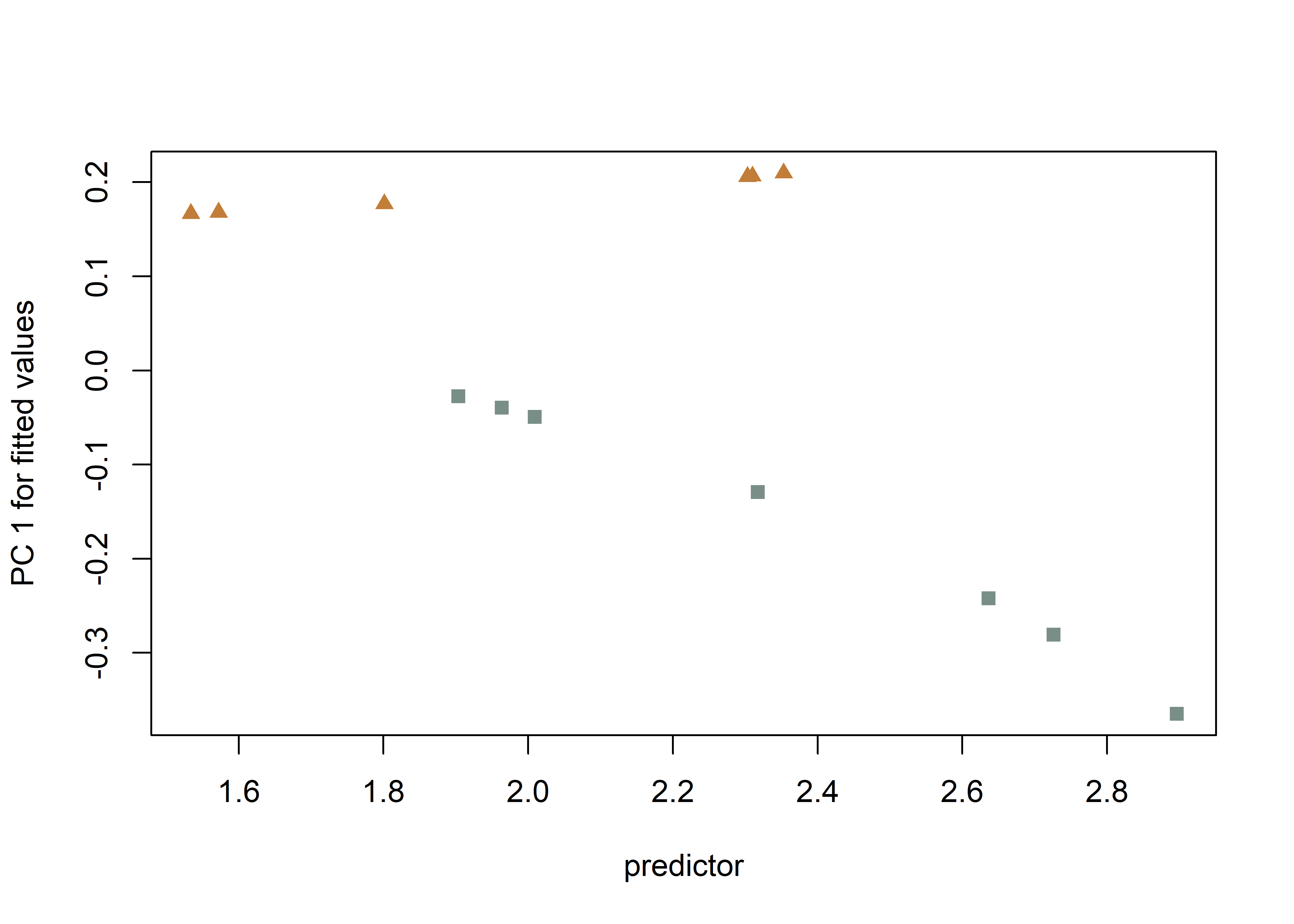
plotAllometry(fit.sz.uinc2,
              size = gdf$size,
              logsz = TRUE,
              method = "PredLine",
              pch = pch.gps.2,
              col = col.gps.2)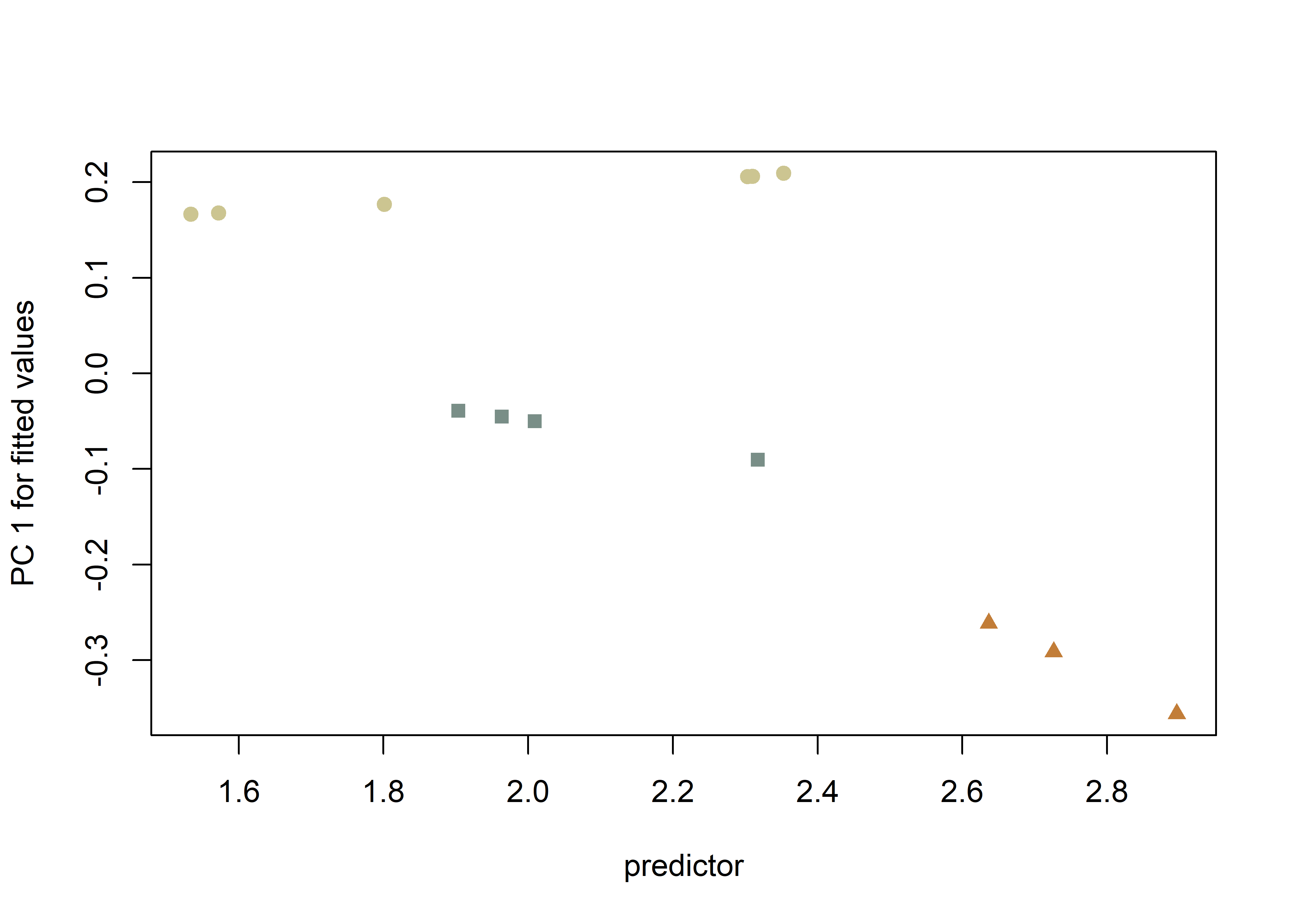
4.6 Size/Shape ~ Incision Profile?
# ANOVA: do incision shapes differ by profile?
anova(fit.shapeinc)
##
## Analysis of Variance, using Residual Randomization
## Permutation procedure: Randomization of null model residuals
## Number of permutations: 10000
## Estimation method: Ordinary Least Squares
## Sums of Squares and Cross-products: Type I
## Effect sizes (Z) based on F distributions
##
## Df SS MS Rsq F Z Pr(>F)
## inc 1 0.40707 0.40707 0.63274 18.951 2.9804 5e-04 ***
## Residuals 11 0.23628 0.02148 0.36726
## Total 12 0.64334
## ---
## Signif. codes: 0 '***' 0.001 '**' 0.01 '*' 0.05 '.' 0.1 ' ' 1
##
## Call: procD.lm(f1 = shape ~ inc, iter = 9999, data = gdf, print.progress = FALSE)# ANOVA: do incision sizes differ by profile?
anova(fit.sizeinc)##
## Analysis of Variance, using Residual Randomization
## Permutation procedure: Randomization of null model residuals
## Number of permutations: 10000
## Estimation method: Ordinary Least Squares
## Sums of Squares and Cross-products: Type I
## Effect sizes (Z) based on F distributions
##
## Df SS MS Rsq F Z Pr(>F)
## inc 1 41.194 41.194 0.20167 2.7787 1.1494 0.1288
## Residuals 11 163.075 14.825 0.79833
## Total 12 204.269
##
## Call: procD.lm(f1 = size ~ inc, iter = 9999, data = gdf, print.progress = FALSE)4.7 Size/Shape ~ Incision Profile 2?
# ANOVA: do incision shapes differ (inc2)?
anova(fit.shapeinc2)
##
## Analysis of Variance, using Residual Randomization
## Permutation procedure: Randomization of null model residuals
## Number of permutations: 10000
## Estimation method: Ordinary Least Squares
## Sums of Squares and Cross-products: Type I
## Effect sizes (Z) based on F distributions
##
## Df SS MS Rsq F Z Pr(>F)
## inc2 2 0.54162 0.270809 0.84188 26.621 3.7921 1e-04 ***
## Residuals 10 0.10173 0.010173 0.15812
## Total 12 0.64334
## ---
## Signif. codes: 0 '***' 0.001 '**' 0.01 '*' 0.05 '.' 0.1 ' ' 1
##
## Call: procD.lm(f1 = shape ~ inc2, iter = 9999, data = gdf, print.progress = FALSE)# pairwise comparison of LS means = which differ?
sh.inc2 <- pairwise(fit.shapeinc2,
groups = qdata$inc2)
summary(sh.inc2,
confidence = 0.95,
test.type = "dist")##
## Pairwise comparisons
##
## Groups: Un Uw V
##
## RRPP: 10000 permutations
##
## LS means:
## Vectors hidden (use show.vectors = TRUE to view)
##
## Pairwise distances between means, plus statistics
## d UCL (95%) Z Pr > d
## Un:Uw 0.2801554 0.3138160 1.412484 0.0885
## Un:V 0.2689149 0.2657416 1.693278 0.0465
## Uw:V 0.4923652 0.2925628 2.848955 0.0001# pairwise distance between variances = standardization?
summary(sh.inc2,
confidence = 0.95,
test.type = "var")##
## Pairwise comparisons
##
## Groups: Un Uw V
##
## RRPP: 10000 permutations
##
##
## Observed variances by group
##
## Un Uw V
## 0.004544256 0.010684141 0.008582835
##
## Pairwise distances between variances, plus statistics
## d UCL (95%) Z Pr > d
## Un:Uw 0.006139884 0.008120517 1.1006324 0.1455
## Un:V 0.004038578 0.006905215 0.6752955 0.2761
## Uw:V 0.002101306 0.007528055 -0.2741477 0.6097# ANOVA: do incision sizes differ (inc2)?
anova(fit.sizeinc2)##
## Analysis of Variance, using Residual Randomization
## Permutation procedure: Randomization of null model residuals
## Number of permutations: 10000
## Estimation method: Ordinary Least Squares
## Sums of Squares and Cross-products: Type I
## Effect sizes (Z) based on F distributions
##
## Df SS MS Rsq F Z Pr(>F)
## inc2 2 148.75 74.374 0.7282 13.396 3.1046 0.0031 **
## Residuals 10 55.52 5.552 0.2718
## Total 12 204.27
## ---
## Signif. codes: 0 '***' 0.001 '**' 0.01 '*' 0.05 '.' 0.1 ' ' 1
##
## Call: procD.lm(f1 = size ~ inc2, iter = 9999, data = gdf, print.progress = FALSE)# pairwise comparison of LS means = which differ?
sz.inc2 <- pairwise(fit.sizeinc2,
groups = qdata$inc2)
summary(sz.inc2,
confidence = 0.95,
test.type = "dist")##
## Pairwise comparisons
##
## Groups: Un Uw V
##
## RRPP: 10000 permutations
##
## LS means:
## Vectors hidden (use show.vectors = TRUE to view)
##
## Pairwise distances between means, plus statistics
## d UCL (95%) Z Pr > d
## Un:Uw 7.9208803 5.971568 2.147324 0.0050
## Un:V 0.1761291 5.062068 -1.724802 0.9510
## Uw:V 8.0970094 5.576685 2.396917 0.0014# pairwise distance between variances = standardization?
summary(sz.inc2,
confidence = 0.95,
test.type = "var")##
## Pairwise comparisons
##
## Groups: Un Uw V
##
## RRPP: 10000 permutations
##
##
## Observed variances by group
##
## Un Uw V
## 1.817578 2.993043 6.545157
##
## Pairwise distances between variances, plus statistics
## d UCL (95%) Z Pr > d
## Un:Uw 1.175464 4.698405 -0.370935 0.6383
## Un:V 4.727578 3.903940 1.952919 0.0160
## Uw:V 3.552114 4.358573 1.220842 0.11854.8 Morphological disparity
# morphological disparity: does incision morphology display greater shape variation among individuals relative to incision profile shape?
morphol.disparity(fit.shapeinc,
                  groups = qdata$inc2,
                  data = gdf,
                  print.progress = FALSE,
                  iter = 9999)
##
## Call:
## morphol.disparity(f1 = fit.shapeinc, groups = qdata$inc2, iter = 9999,
## data = gdf, print.progress = FALSE)
##
##
##
## Randomized Residual Permutation Procedure Used
## 10000 Permutations
##
## Procrustes variances for defined groups
## Un Uw V
## 0.018960247 0.036312568 0.008582835
##
##
## Pairwise absolute differences between variances
## Un Uw V
## Un 0.00000000 0.01735232 0.01037741
## Uw 0.01735232 0.00000000 0.02772973
## V 0.01037741 0.02772973 0.00000000
##
##
## P-Values
## Un Uw V
## Un 1.0000 0.2677 0.4830
## Uw 0.2677 1.0000 0.0205
## V 0.4830 0.0205 1.0000# morphological disparity: does incision morphology display greater size variation among individuals relative to incision profile size?
morphol.disparity(fit.sizeinc,
groups = qdata$inc2,
data = gdf,
print.progress = FALSE,
iter = 9999)##
## Call:
## morphol.disparity(f1 = fit.sizeinc, groups = qdata$inc2, iter = 9999,
## data = gdf, print.progress = FALSE)
##
##
##
## Randomized Residual Permutation Procedure Used
## 10000 Permutations
##
## Procrustes variances for defined groups
## Un Uw V
## 13.341315 23.479686 6.545157
##
##
## Pairwise absolute differences between variances
## Un Uw V
## Un 0.000000 10.13837 6.796158
## Uw 10.138371 0.00000 16.934529
## V 6.796158 16.93453 0.000000
##
##
## P-Values
## Un Uw V
## Un 1.0000 0.2941 0.4539
## Uw 0.2941 1.0000 0.0255
## V 0.4539 0.0255 1.00004.9 Mean shapes
# subset landmark coordinates to produce mean shapes by site
new.coords <- coords.subset(A = Y.gpa$coords,
                            group = qdata$inc2)

names(new.coords)
## [1] "Un" "Uw" "V"# group shape means
mean <- lapply(new.coords, mshape)
# plot(mean$Uw)
# mean shapes
knitr::include_graphics('images/mshapeEX.png')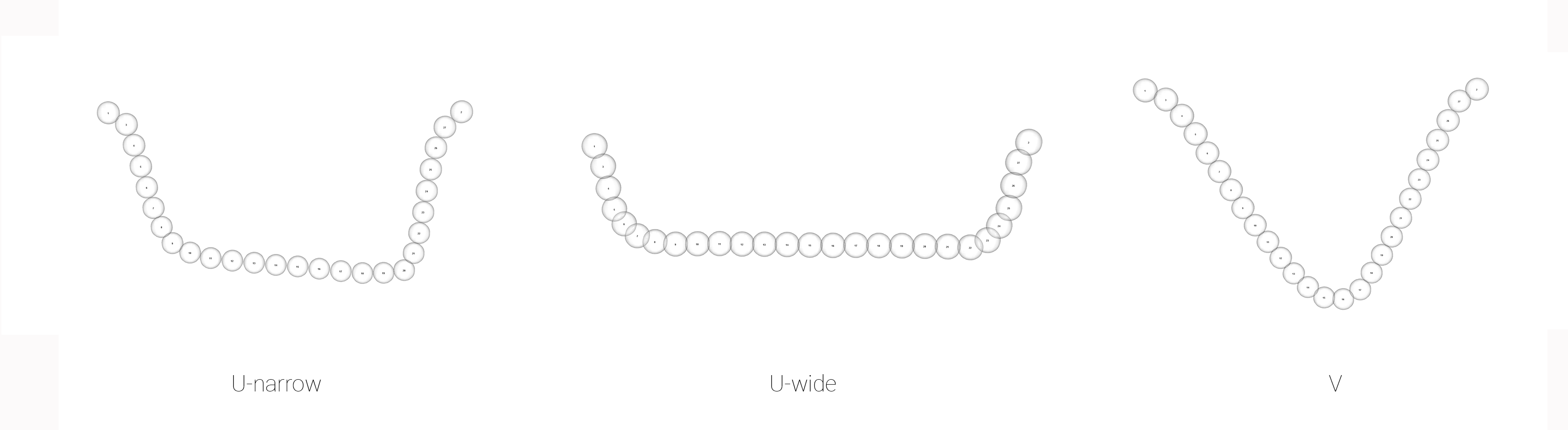
Figure 4.6: Mean shapes for incision profiles Un, Uw, and V.