Chapter 2 Landmarking protocol
The characteristic points and tangents used in this landmarking protocol were inspired by the pioneering work of Birkhoff (1933). The final configuration employs two landmarks—one at each horizontal tangent—with an additional 25 equidistant semilandmarks placed along the dynamic contours of the spline.
2.1 Calculating depth
The method of calculating the depth of each incision employed the use of two planes. One plane was placed on the surface of each sherd using six points, with three on either side of the incision. The second plane was inserted using the offset function, and was extended to the furthest extent of the mesh associated with the incision. A reference point was inserted at that location, providing the X-coordinate of the cross-section.
2.2 Placing the landmarks
Using Geomagic Design X, a plane was inserted at the location of the reference point to capture the deepest incision profile. The rationale behind selecting the deepest incision profile is that these marks were made when the vessel was not yet leather hard, and the deepest incision would provide the most complete cross-section of the tool used in the application of the decorative motif.
# incision image
knitr::include_graphics('images/insertplane.png')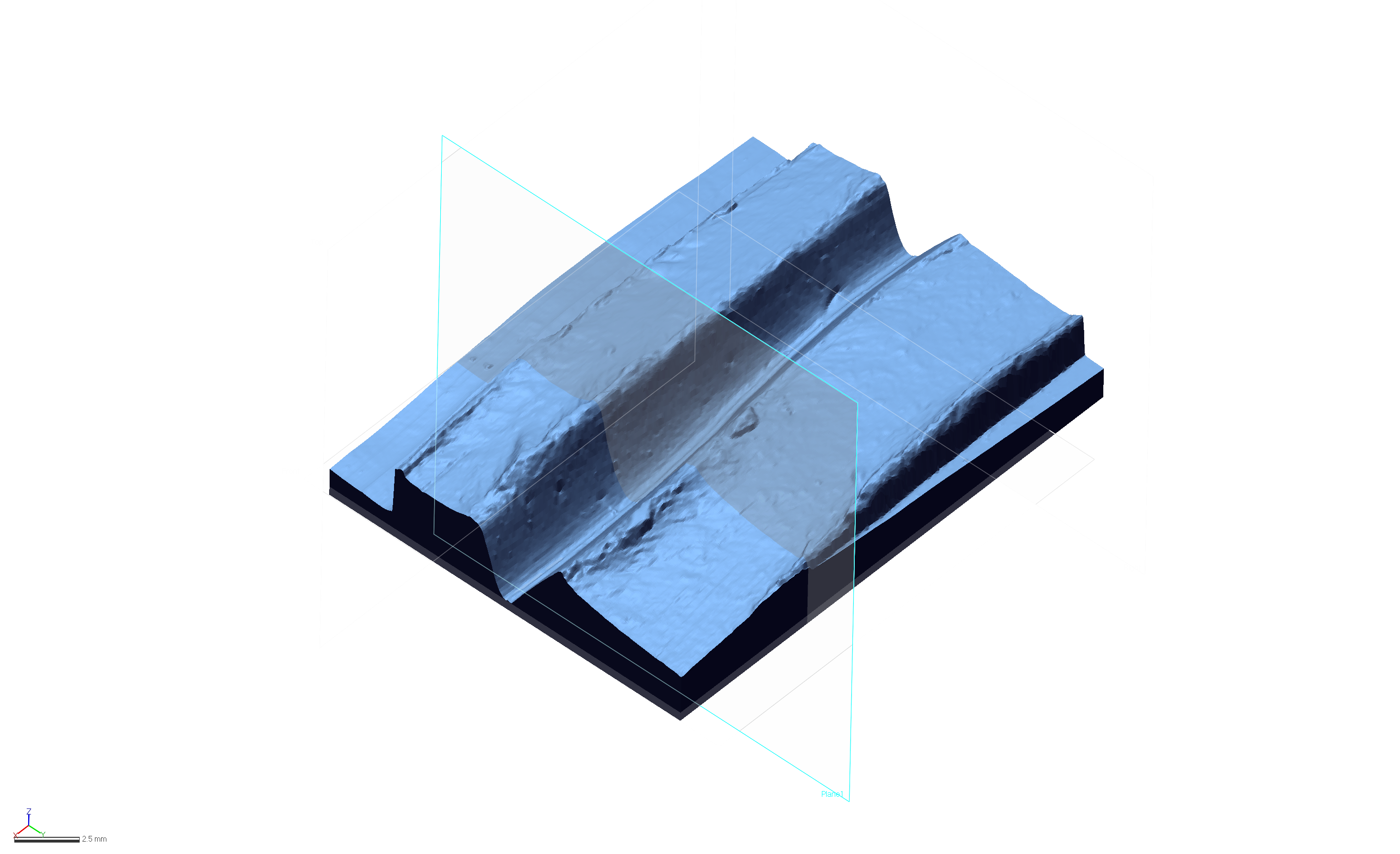
fig.cap="Reference plane (blue) inserted at deepest point of incision of experimental tile 6b."After isolating the profile of the incision, the horizontal tangent was identified for the rise in the clay matrix above the reference plane on either side, then calculation of the linear distance between the tangents to identify the mid-point. Prior to the application of landmarks, the deepest point of the incision profile (X-coordinate) was oriented to the right of center.
# incision image
knitr::include_graphics('images/h-tangents.png')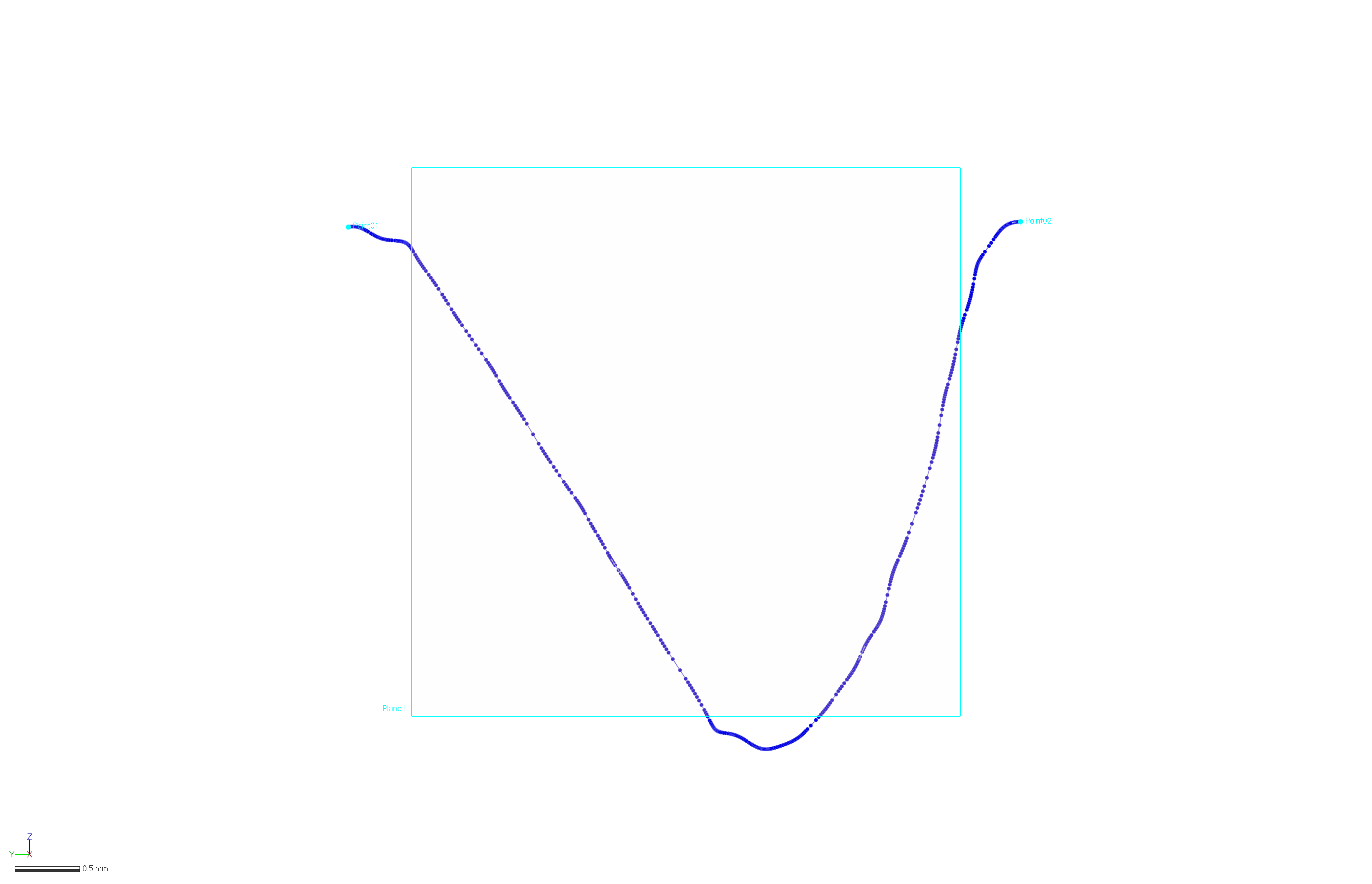
fig.cap="Spline (500 interpolation points) that was cut at the location of horizontal tangents on each side, then oriented where the deepest part of the incision was to the right of center."Once properly oriented, the horizontal tangent on the left was assigned as landmark (LM) 01, and the tangent on the right as LM 02. Twenty five equidistant landmarks were inserted between the two landmarks along the spline.
# incision image
knitr::include_graphics('images/semiland.png')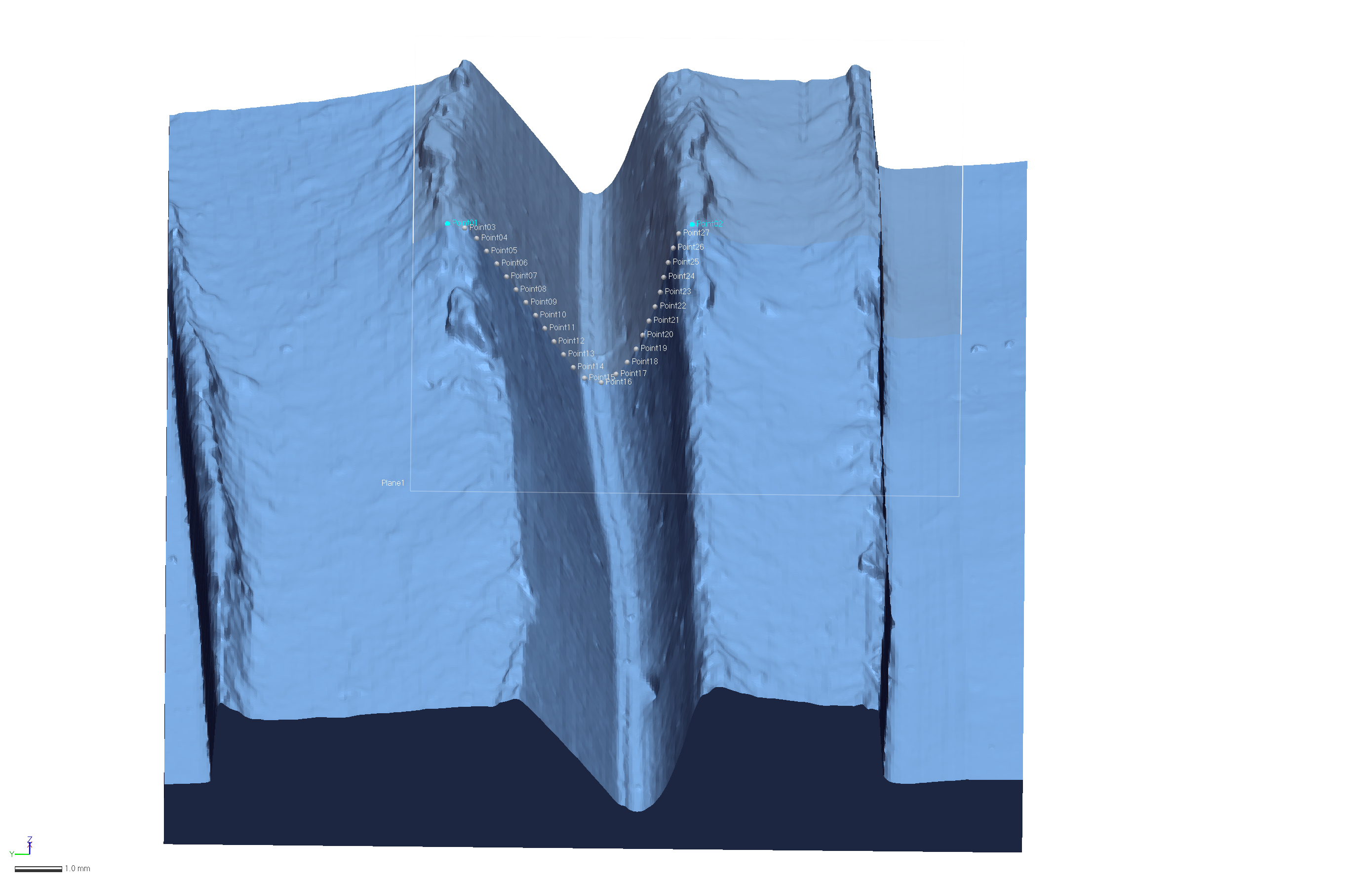
fig.cap="Placement of 25 equidistant semilandmarks (white) between LM01 and LM02 (blue)"Landmarks and semilandmarks associated with each specimen were then exported as CSV files. These are included in the supplemental materials as dataEX for the experimental sample, and data1 for the archaeological sample.